


One-Pole
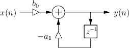
Fig.B.3 gives the signal flow graph for the general one-pole filter. The road to the frequency response goes as follows:
 |
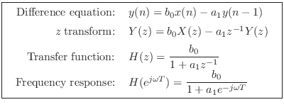
The one-pole filter has a transfer function (hence frequency response) which is the reciprocal of that of a one-zero. The analysis is thus quite analogous. The frequency response in polar form is given by
![\begin{eqnarray*}
G(\omega) &=& \frac{\vert b_0\vert}{\sqrt{[1 + a_1 \cos(\omega...
... + a_1 \cos(\omega T)}\right], & b_0<0 \\
\end{array} \right..
\end{eqnarray*}](http://www.dsprelated.com/josimages_new/filters/img1351.png)
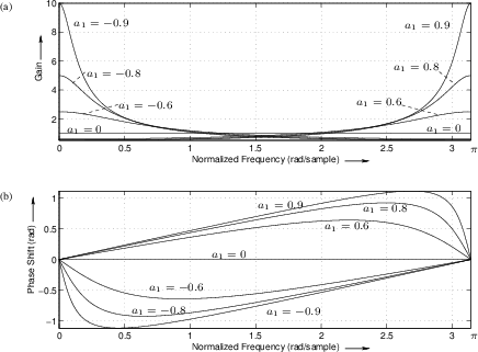
A plot of the frequency response in polar form for ![]() and
various values of
and
various values of ![]() is given in Fig.B.4.
is given in Fig.B.4.
The filter has a pole at ![]() , in the
, in the ![]() plane (and a zero at
plane (and a zero at ![]() = 0). Notice that the one-pole exhibits
either a lowpass or a highpass frequency response, like the
one-zero. The lowpass character occurs when the pole is near the point
= 0). Notice that the one-pole exhibits
either a lowpass or a highpass frequency response, like the
one-zero. The lowpass character occurs when the pole is near the point
![]() (dc), which happens when
(dc), which happens when ![]() approaches
approaches ![]() . Conversely,
the highpass nature occurs when
. Conversely,
the highpass nature occurs when ![]() is positive.
is positive.
The one-pole filter section can achieve much more drastic differences
between the gain at high frequencies and the gain at low frequencies
than can the one-zero filter. This difference is achieved in the
one-pole by gain boost in the passband rather than
attenuation in the stopband; thus it is usually desirable when
using a one-pole filter to set ![]() to a small value, such as
to a small value, such as
![]() , so that the peak gain is 1 or so. When the peak gain is 1,
the filter is unlikely to overflow.B.1
, so that the peak gain is 1 or so. When the peak gain is 1,
the filter is unlikely to overflow.B.1
Finally, note that the one-pole filter is stable if and only if
![]() .
.
Next Section:
Two-Pole
Previous Section:
One-Zero


