


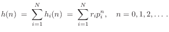
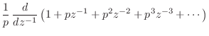
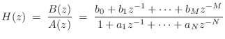
Transfer Function Analysis
This chapter discusses filter transfer functions and associated analysis. The transfer function provides an algebraic representation of a linear, time-invariant (LTI) filter in the frequency domain:
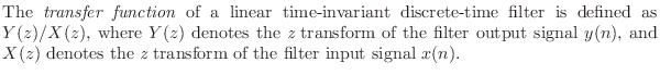
The transfer function is also called the system function [60].
Let ![]() denote the impulse response of the filter. It turns
out (as we will show) that the transfer function is equal to the
z transform of the impulse response
denote the impulse response of the filter. It turns
out (as we will show) that the transfer function is equal to the
z transform of the impulse response ![]() :
:
It remains to define ``z transform'', and to prove that the z transform of the impulse response always gives the transfer function, which we will do by proving the convolution theorem for z transforms.
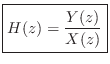
The Z Transform
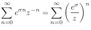
The bilateral z transform of the discrete-time signal ![]() is
defined to be
is
defined to be
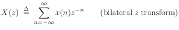
where
 |
(7.2) |
The unilateral z transform is most commonly used. For inverting z transforms, see §6.8.
Recall (§4.1) that the mathematical representation of a
discrete-time signal ![]() maps each integer
maps each integer
![]() to a complex
number (
to a complex
number (
![]() ) or real number (
) or real number (
![]() ). The z transform
of
). The z transform
of ![]() , on the other hand,
, on the other hand, ![]() , maps every complex number
, maps every complex number
![]() to a new complex number
to a new complex number
![]() . On a higher
level, the z transform, viewed as a linear operator, maps an entire
signal
. On a higher
level, the z transform, viewed as a linear operator, maps an entire
signal ![]() to its z transform
to its z transform ![]() . We think of this as a ``function to
function'' mapping. We may say
. We think of this as a ``function to
function'' mapping. We may say ![]() is the z transform of
is the z transform of ![]() by writing
by writing
The z transform of a signal ![]() can be regarded as a polynomial in
can be regarded as a polynomial in
![]() , with coefficients given by the signal samples. For example,
the signal
, with coefficients given by the signal samples. For example,
the signal
![$\displaystyle x(n) = \left\{\begin{array}{ll}
n+1, & 0\leq n \leq 2 \\ [5pt]
0, & \mbox{otherwise} \\
\end{array}\right.
$](http://www.dsprelated.com/josimages_new/filters/img633.png)
Existence of the Z Transform
The z transform of a finite-amplitude
signal ![]() will always exist provided (1) the signal starts at a finite time and (2) it is
asymptotically exponentially bounded, i.e., there exists a
finite integer
will always exist provided (1) the signal starts at a finite time and (2) it is
asymptotically exponentially bounded, i.e., there exists a
finite integer ![]() , and finite real numbers
, and finite real numbers ![]() and
and ![]() ,
such that
,
such that
![]() for all
for all ![]() . The
bounding exponential may even be growing with
. The
bounding exponential may even be growing with ![]() (
(![]() ). These are
not the most general conditions for existence of the z transform, but they
suffice for most practical purposes.
). These are
not the most general conditions for existence of the z transform, but they
suffice for most practical purposes.
For a signal ![]() growing as
growing as
![]() , for
, for ![]() , one
would naturally expect the z transform
, one
would naturally expect the z transform ![]() to be defined only in the
region
to be defined only in the
region
![]() of the complex plane. This is expected
because the infinite series
of the complex plane. This is expected
because the infinite series
More generally, it turns out that, in all cases of practical interest,
the domain of ![]() can be extended to include the
entire complex plane, except at isolated ``singular''
points7.2 at which
can be extended to include the
entire complex plane, except at isolated ``singular''
points7.2 at which ![]() approaches
infinity (such as at
approaches
infinity (such as at
![]() when
when
![]() ).
The mathematical technique for doing this is called analytic
continuation, and it is described in §D.1 as applied to the
Laplace transform (the continuous-time counterpart of the z transform).
A point to note, however, is that in the extension region (all points
).
The mathematical technique for doing this is called analytic
continuation, and it is described in §D.1 as applied to the
Laplace transform (the continuous-time counterpart of the z transform).
A point to note, however, is that in the extension region (all points
![]() such that
such that
![]() in the above example), the signal
component corresponding to each singularity inside the extension
region is ``flipped'' in the time domain. That is, ``causal''
exponentials become ``anticausal'' exponentials, as discussed in
§8.7.
in the above example), the signal
component corresponding to each singularity inside the extension
region is ``flipped'' in the time domain. That is, ``causal''
exponentials become ``anticausal'' exponentials, as discussed in
§8.7.
The z transform is discussed more fully elsewhere [52,60], and we will derive below only what we will need.
Shift and Convolution Theorems
In this section, we prove the highly useful shift theorem and
convolution theorem for unilateral z transforms. We consider the space of
infinitely long, causal, complex sequences
![]() ,
,
![]() , with
, with ![]() for
for ![]() .
.
Shift Theorem
The shift theorem says that a delay of ![]() samples
in the time domain corresponds to a multiplication by
samples
in the time domain corresponds to a multiplication by
![]() in the frequency domain:
in the frequency domain:
Proof:
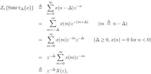
where we used the causality assumption ![]() for
for ![]() .
.
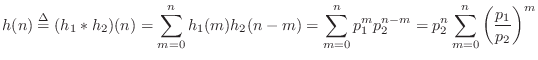
Convolution Theorem
The convolution theorem for z transforms states that for any (real or)
complex causal signals ![]() and
and ![]() ,
convolution in the time domain is multiplication in the
,
convolution in the time domain is multiplication in the
![]() domain, i.e.,
domain, i.e.,
Proof:
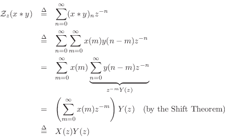
The convolution theorem provides a major cornerstone of linear systems theory. It implies, for example, that any stable causal LTI filter (recursive or nonrecursive) can be implemented by convolving the input signal with the impulse response of the filter, as shown in the next section.
Z Transform of Convolution
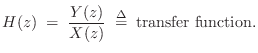
From Eq.![]() (5.5), we have that the output
(5.5), we have that the output ![]() from a linear
time-invariant filter with input
from a linear
time-invariant filter with input ![]() and impulse response
and impulse response ![]() is given
by the convolution of
is given
by the convolution of ![]() and
and ![]() , i.e.,
, i.e.,
where ``
where H(z) is the z transform of the filter impulse response. We may divide Eq.
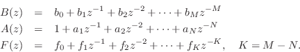
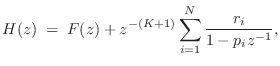
Z Transform of Difference Equations
Since z transforming the convolution representation for digital filters was
so fruitful, let's apply it now to the general difference equation,
Eq.![]() (5.1). To do this requires two properties of the z transform,
linearity (easy to show) and the shift theorem
(derived in §6.3 above). Using these two properties, we
can write down the z transform of any difference equation by inspection, as
we now show. In
§6.8.2, we'll show how to invert by inspection as well.
(5.1). To do this requires two properties of the z transform,
linearity (easy to show) and the shift theorem
(derived in §6.3 above). Using these two properties, we
can write down the z transform of any difference equation by inspection, as
we now show. In
§6.8.2, we'll show how to invert by inspection as well.
Repeating the general difference equation for LTI filters, we have
(from Eq.![]() (5.1))
(5.1))

Let's take the z transform of both sides, denoting the transform by
![]() . Because
. Because
![]() is a linear operator,
it may be distributed through the terms on the right-hand side as
follows:7.3
is a linear operator,
it may be distributed through the terms on the right-hand side as
follows:7.3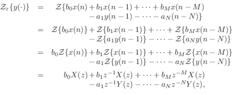 where we used the superposition and scaling properties of linearity
given on page
where we used the superposition and scaling properties of linearity
given on page ![]() , followed by use of the shift
theorem, in that order. The terms in
, followed by use of the shift
theorem, in that order. The terms in ![]() may be grouped together
on the left-hand side to get
may be grouped together
on the left-hand side to get

Factoring out the common terms ![]() and
and ![]() gives
gives

the z transform of the difference equation yields
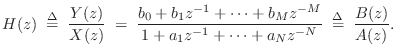
Thus, taking the z transform of the general difference equation led to a new formula for the transfer function in terms of the difference equation coefficients. (Now the minus signs for the feedback coefficients in the difference equation Eq.
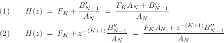
Factored Form
By the fundamental theorem of algebra, every ![]() th order polynomial
can be factored into a product of
th order polynomial
can be factored into a product of ![]() first-order polynomials.
Therefore, Eq.
first-order polynomials.
Therefore, Eq.![]() (6.5) above can be written in
factored form as
(6.5) above can be written in
factored form as
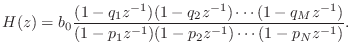
The numerator roots
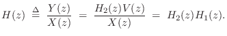
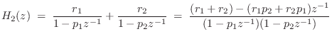
Series and Parallel Transfer Functions
The transfer function conveniently captures the algebraic structure of a filtering operation with respect to series or parallel combination. Specifically, we have the following cases:
- Transfer functions of filters in series multiply together.
- Transfer functions of filters in parallel sum together.
Series Case
Figure 6.1 illustrates the series connection of two
filters
![]() and
and
![]() .
The output
.
The output ![]() from filter 1 is used as the input to filter 2.
Therefore, the overall transfer function is
from filter 1 is used as the input to filter 2.
Therefore, the overall transfer function is
Parallel Case
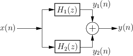
Figure 6.2 illustrates the parallel combination of two
filters. The filters ![]() and
and ![]() are driven by the
same input signal
are driven by the
same input signal ![]() , and their respective outputs
, and their respective outputs ![]() and
and ![]() are summed. The transfer function of the parallel
combination is therefore
are summed. The transfer function of the parallel
combination is therefore

Series Combination is Commutative
Since multiplication of complex numbers is commutative, we have
By the convolution theorem for z transforms, commutativity of a product of transfer functions implies that convolution is commutative:
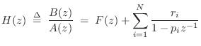
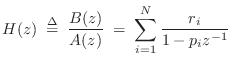
Partial Fraction Expansion
An important tool for inverting the z transform and converting among digital filter implementation structures is the partial fraction expansion (PFE). The term ``partial fraction expansion'' refers to the expansion of a rational transfer function into a sum of first and/or second-order terms. The case of first-order terms is the simplest and most fundamental:
where
and ![]() . (The case
. (The case ![]() is addressed in the next section.)
The denominator coefficients
is addressed in the next section.)
The denominator coefficients ![]() are called the poles of the
transfer function, and each numerator
are called the poles of the
transfer function, and each numerator ![]() is called the
residue of pole
is called the
residue of pole ![]() . Equation (6.7) is general only if the poles
. Equation (6.7) is general only if the poles
![]() are distinct. (Repeated poles are addressed in
§6.8.5 below.) Both the poles and their residues may be
complex. The poles may be found by factoring the polynomial
are distinct. (Repeated poles are addressed in
§6.8.5 below.) Both the poles and their residues may be
complex. The poles may be found by factoring the polynomial ![]() into first-order terms,7.4e.g., using the roots function in matlab.
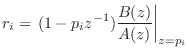
The residue
into first-order terms,7.4e.g., using the roots function in matlab.
The residue ![]() corresponding to pole
corresponding to pole ![]() may be found
analytically as
may be found
analytically as
when the poles
Note that in Eq.![]() (6.8), there is always a pole-zero cancellation at
(6.8), there is always a pole-zero cancellation at
![]() . That is, the term
. That is, the term
![]() is always cancelled by an
identical term in the denominator of
is always cancelled by an
identical term in the denominator of ![]() , which must exist because
, which must exist because
![]() has a pole at
has a pole at ![]() . The residue
. The residue ![]() is simply the
coefficient of the one-pole term
is simply the
coefficient of the one-pole term
![]() in the partial
fraction expansion of
in the partial
fraction expansion of ![]() at
at ![]() . The transfer function
is
. The transfer function
is
![]() , in the limit, as
, in the limit, as ![]() .
.
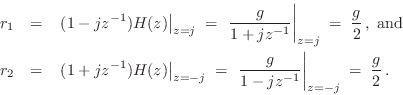
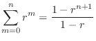
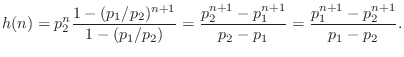
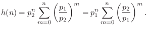
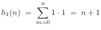
Example
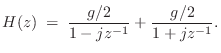
Consider the two-pole filter
We thus conclude that
Complex Example
To illustrate an example involving complex poles, consider the filter
Thus,
A more elaborate example of a partial fraction expansion into complex one-pole sections is given in §3.12.1.
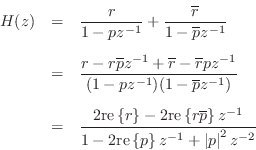
PFE to Real, Second-Order Sections
When all coefficients of ![]() and
and ![]() are real (implying that
are real (implying that
![]() is the transfer function of
a real filter), it will
always happen that the complex one-pole filters will occur in
complex conjugate pairs. Let
is the transfer function of
a real filter), it will
always happen that the complex one-pole filters will occur in
complex conjugate pairs. Let ![]() denote any one-pole
section in the PFE of Eq.
denote any one-pole
section in the PFE of Eq.![]() (6.7). Then if
(6.7). Then if ![]() is complex and
is complex and ![]() describes a real filter, we will also find
describes a real filter, we will also find
![]() somewhere among
the terms in the one-pole expansion. These two terms can be paired to
form a real second-order section as follows:
somewhere among
the terms in the one-pole expansion. These two terms can be paired to
form a real second-order section as follows:
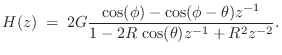
Expressing the pole ![]() in polar form as
in polar form as
![]() ,
and the residue as
,
and the residue as
![]() ,
the last expression above can be rewritten as
,
the last expression above can be rewritten as
Expanding a transfer function into a sum of second-order terms with
real coefficients gives us the filter coefficients for a parallel bank
of real second-order filter sections. (Of course, each real pole can
be implemented in its own real one-pole section in parallel with the
other sections.) In view of the foregoing, we may conclude that every
real filter with ![]() can be implemented as a parallel bank
of biquads.7.6 However, the full generality of a biquad
section (two poles and two zeros) is not needed because the PFE
requires only one zero per second-order term.
can be implemented as a parallel bank
of biquads.7.6 However, the full generality of a biquad
section (two poles and two zeros) is not needed because the PFE
requires only one zero per second-order term.
To see why we must stipulate ![]() in Eq.
in Eq.![]() (6.7), consider the sum of two
first-order terms by direct calculation:
(6.7), consider the sum of two
first-order terms by direct calculation:
 |
(7.9) |
Notice that the numerator order, viewed as a polynomial in
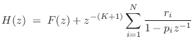
Inverting the Z Transform
The partial fraction expansion (PFE) provides a simple means for inverting the z transform of rational transfer functions. The PFE provides a sum of first-order terms of the form
In the improper case, discussed in the next section, we additionally obtain an FIR part in the z transform to be inverted:
The case of repeated poles is addressed in §6.8.5 below.
FIR Part of a PFE
When ![]() in Eq.
in Eq.![]() (6.7), we may perform a step of long division
of
(6.7), we may perform a step of long division
of ![]() to produce an FIR part in parallel with a
strictly proper IIR part:
to produce an FIR part in parallel with a
strictly proper IIR part:
where
When ![]() , we define
, we define ![]() . This type of decomposition is
computed by the residuez function (a matlab function for
computing a complete partial fraction expansion, as illustrated in
§6.8.8 below).
. This type of decomposition is
computed by the residuez function (a matlab function for
computing a complete partial fraction expansion, as illustrated in
§6.8.8 below).
An alternate FIR part is obtained by performing long division on the reversed polynomial coefficients to obtain
where
We may compare these two PFE alternatives as follows:
Let ![]() denote
denote ![]() ,
,
![]() , and
, and
![]() .
(I.e., we use a subscript to indicate polynomial order, and `
.
(I.e., we use a subscript to indicate polynomial order, and `![]() ' is
omitted for notational simplicity.) Then for
' is
omitted for notational simplicity.) Then for
![]() we have two cases:
we have two cases:
In the first form, the
![]() coefficients are ``left
justified'' in the reconstructed numerator, while in the second form
they are ``right justified''. The second form is generally more
efficient for modeling purposes, since the numerator of the IIR
part (
coefficients are ``left
justified'' in the reconstructed numerator, while in the second form
they are ``right justified''. The second form is generally more
efficient for modeling purposes, since the numerator of the IIR
part (
![]() ) can be used to match additional
terms in the impulse response after the FIR part
) can be used to match additional
terms in the impulse response after the FIR part ![]() has
``died out''.
has
``died out''.
In summary, an arbitrary digital filter transfer function ![]() with
with
![]() distinct poles can always be expressed as a parallel combination
of complex one-pole filters, together with a parallel FIR part
when
distinct poles can always be expressed as a parallel combination
of complex one-pole filters, together with a parallel FIR part
when ![]() . When there is an FIR part, the strictly proper IIR
part may be delayed such that its impulse response begins where that
of the FIR part leaves off.
. When there is an FIR part, the strictly proper IIR
part may be delayed such that its impulse response begins where that
of the FIR part leaves off.
In artificial reverberation applications, the FIR part may correspond to the early reflections, while the IIR part provides the late reverb, which is typically dense, smooth, and exponentially decaying [86]. The predelay (``pre-delay'') control in some commercial reverberators is the amount of pure delay at the beginning of the reverberator's impulse response. Thus, neglecting the early reflections, the order of the FIR part can be viewed as the amount of predelay for the IIR part.
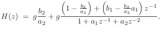
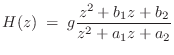
Example: The General Biquad PFE
The general second-order case with ![]() (the so-called
biquad section) can be written when
(the so-called
biquad section) can be written when ![]() as
as

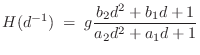

yielding
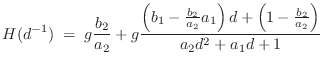
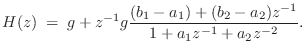
The delayed form of the partial fraction expansion is obtained by
leaving the coefficients in their original order. This corresponds
to writing ![]() as a ratio of polynomials in
as a ratio of polynomials in ![]() :
:

giving
Numerical examples of partial fraction expansions are given in §6.8.8
below. Another worked example, in which the filter
![]() is converted to a set of parallel, second-order
sections is given in §3.12. See also §9.2 regarding
conversion to second-order sections in general, and §G.9.1 (especially
Eq.
is converted to a set of parallel, second-order
sections is given in §3.12. See also §9.2 regarding
conversion to second-order sections in general, and §G.9.1 (especially
Eq.![]() (G.22)) regarding
a state-space approach to partial fraction expansion.
(G.22)) regarding
a state-space approach to partial fraction expansion.
Alternate PFE Methods
Another method for finding the pole residues is to write down the general
form of the PFE, obtain a common denominator, expand the numerator
terms to obtain a single polynomial, and equate like powers of ![]() .
This gives a linear system of
.
This gives a linear system of ![]() equations in
equations in ![]() unknowns
unknowns ![]() ,
,
![]() .
.
Yet another method for finding residues is by means of Taylor series
expansions of the numerator ![]() and denominator
and denominator ![]() about each
pole
about each
pole ![]() , using l'Hôpital's
rule..
, using l'Hôpital's
rule..
Finally, one can alternatively construct a state space realization of a strictly proper transfer function (using, e.g., tf2ss in matlab) and then diagonalize it via a similarity transformation. (See Appendix G for an introduction to state-space models and diagonalizing them via similarity transformations.) The transfer function of the diagonalized state-space model is trivially obtained as a sum of one-pole terms--i.e., the PFE. In other words, diagonalizing a state-space filter realization implicitly performs a partial fraction expansion of the filter's transfer function. When the poles are distinct, the state-space model can be diagonalized; when there are repeated poles, it can be block-diagonalized instead, as discussed further in §G.10.
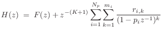
Repeated Poles
When poles are repeated, an interesting new phenomenon emerges. To see what's going on, let's consider two identical poles arranged in parallel and in series. In the parallel case, we have
Dealing with Repeated Poles Analytically
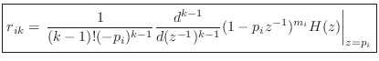
A pole of multiplicity ![]() has
has
![]() residues associated with it. For example,
residues associated with it. For example,
and the three residues associated with the pole
Let ![]() denote the
denote the ![]() th residue associated with the pole
th residue associated with the pole ![]() ,
,
![]() .
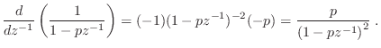
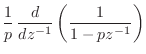
Successively differentiating
.
Successively differentiating
![]()
![]() times with
respect to
times with
respect to ![]() and setting
and setting ![]() isolates the residue
isolates the residue ![]() :
:
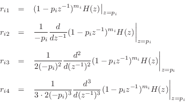
or
Example
For the example of Eq.![]() (6.12), we obtain
(6.12), we obtain

Impulse Response of Repeated Poles
In the time domain, repeated poles give rise to polynomial amplitude envelopes on the decaying exponentials corresponding to the (stable) poles. For example, in the case of a single pole repeated twice, we have

Proof:
First note that
 |
|||
 |
|||
 |
|||
| (7.13) |
Note that
So What's Up with Repeated Poles?
In the previous section, we found that repeated poles give rise to polynomial amplitude-envelopes multiplying the exponential decay due to the pole. On the other hand, two different poles can only yield a convolution (or sum) of two different exponential decays, with no polynomial envelope allowed. This is true no matter how closely the poles come together; the polynomial envelope can occur only when the poles merge exactly. This might violate one's intuitive expectation of a continuous change when passing from two closely spaced poles to a repeated pole.
To study this phenomenon further, consider the convolution of two
one-pole impulse-responses
![]() and
and
![]() :
:
The finite limits on the summation result from the fact that both
Going back to Eq.![]() (6.14), we have
(6.14), we have
 |
(7.15) |
Setting
| (7.16) |
which is the first-order polynomial amplitude-envelope case for a repeated pole. We can see that the transition from ``two convolved exponentials'' to ``single exponential with a polynomial amplitude envelope'' is perfectly continuous, as we would expect.
We also see that the polynomial amplitude-envelopes fundamentally
arise from iterated convolutions. This corresponds to the
repeated poles being arranged in series, rather than in
parallel. The simplest case is when the repeated pole is at ![]() , in
which case its impulse response is a constant:
, in
which case its impulse response is a constant:

Alternate Stability Criterion
In §5.6 (page ![]() ), a filter was defined to
be stable if its impulse response
), a filter was defined to
be stable if its impulse response ![]() decays to 0 in
magnitude as time
decays to 0 in
magnitude as time ![]() goes to infinity. In §6.8.5, we saw that
the impulse response of every finite-order LTI filter can be expressed
as a possible FIR part (which is always stable) plus a linear
combination of terms of the form
goes to infinity. In §6.8.5, we saw that
the impulse response of every finite-order LTI filter can be expressed
as a possible FIR part (which is always stable) plus a linear
combination of terms of the form
![]() , where
, where ![]() is some
finite-order polynomial in
is some
finite-order polynomial in ![]() , and
, and ![]() is the
is the ![]() th pole of the
filter. In this form, it is clear that the impulse response always
decays to zero when each pole is strictly inside the unit circle of
the
th pole of the
filter. In this form, it is clear that the impulse response always
decays to zero when each pole is strictly inside the unit circle of
the ![]() plane, i.e., when
plane, i.e., when ![]() . Thus, having all poles strictly
inside the unit circle is a sufficient criterion for filter
stability. If the filter is observable (meaning that there are
no pole-zero cancellations in the transfer function from input to
output), then this is also a necessary criterion.
. Thus, having all poles strictly
inside the unit circle is a sufficient criterion for filter
stability. If the filter is observable (meaning that there are
no pole-zero cancellations in the transfer function from input to
output), then this is also a necessary criterion.
A transfer function with no pole-zero cancellations is said to be
irreducible. For example,
![]() is
irreducible, while
is
irreducible, while
![]() is reducible, since
there is the common factor of
is reducible, since
there is the common factor of
![]() in the numerator and
denominator. Using this terminology, we may state the following
stability criterion:
in the numerator and
denominator. Using this terminology, we may state the following
stability criterion:
This characterization of stability is pursued further in §8.4, and yet another stability test (most often used in practice) is given in §8.4.1.
Summary of the Partial Fraction Expansion
In summary, the partial fraction expansion can be used to expand any rational z transform
 |
(7.17) |
for
for
- When
 , perform a step of long division to obtain
an FIR part
, perform a step of long division to obtain
an FIR part  and a strictly proper IIR part
 .
.
- Find the
 poles
poles  ,
,
 (roots of
  ).
).
- If the poles are distinct, find the residues
 ,
from
,
from
- If there are repeated poles, find the additional residues via
the method of §6.8.5, and the general form of the PFE is
where denotes the number of distinct poles, and
 denotes the multiplicity of the
  th pole.
In step 2, the poles are typically found by factoring the
denominator polynomial ![]() . This is a dangerous step numerically
which may fail when there are many poles, especially when many poles
are clustered close together in the
. This is a dangerous step numerically
which may fail when there are many poles, especially when many poles
are clustered close together in the ![]() plane.
plane.
The following matlab code illustrates factoring
![]() to
obtain the three roots,
to
obtain the three roots,
![]() ,
, ![]() :
:
A = [1 0 0 -1];  % Filter denominator polynomial
poles = roots(A) % Filter poles
See Chapter 9 for additional discussion regarding digital filters implemented as parallel sections (especially §9.2.2).
Software for Partial Fraction Expansion
Figure 6.3 illustrates the use of residuez (§J.5) for performing a partial fraction expansion on the transfer function
B = [1 0 0 0.125]; A = [1 0 0 0 0 0.9^5]; [r,p,f] = residuez(B,A) % r = % 0.16571 % 0.22774 - 0.02016i % 0.22774 + 0.02016i % 0.18940 + 0.03262i % 0.18940 - 0.03262i % % p = % -0.90000 % -0.27812 - 0.85595i % -0.27812 + 0.85595i % 0.72812 - 0.52901i % 0.72812 + 0.52901i % % f = [](0x0) |
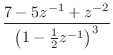
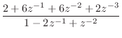
Example 2
For the filter
![$\displaystyle (2+10z^{-1}) + z^{-2}\left[\frac{8}{1-z^{-1}} + \frac{16}{(1-z^{-1})^2}\right]
\protect$](http://www.dsprelated.com/josimages_new/filters/img819.png)
we obtain the output of residued (§J.6) shown in Fig.6.4. In contrast to residuez, residued delays the IIR part until after the FIR part. In contrast to this result, residuez returns r=[-24;16] and f=[10;2], corresponding to the PFE
| (7.22) |
in which the FIR and IIR parts have overlapping impulse responses.
See Sections J.5 and J.6 starting on page ![]() for
listings of residuez, residued and related
discussion.
for
listings of residuez, residued and related
discussion.
B=[2 6 6 2]; A=[1 -2 1]; [r,p,f,m] = residued(B,A) % r = % 8 % 16 % % p = % 1 % 1 % % f = % 2 10 % % m = % 1 % 2 |
Polynomial Multiplication in Matlab
The matlab function conv (convolution) can be used to perform polynomial multiplication. For example:
B1 = [1 1];   % 1st row of Pascal's triangle
B2 = [1 2 1]; % 2nd row of Pascal's triangle
B3 = conv(B1,B2) % 3rd row
% B3 = 1  3  3  1
B4 = conv(B1,B3) % 4th row
% B4 = 1  4  6  4  1
% ...
The matlab conv(B1,B2) is identical to filter(B1,1,B2), except that conv returns the complete convolution of its two input vectors, while filter truncates the result to the length of the ``input signal'' B2.7.10 Thus, if B2 is zero-padded with length(B1)-1 zeros, it will return the complete convolution:
B1 = [1 2 3];
B2 = [4 5 6 7];
conv(B1,B2)
% ans = 4  13  28  34  32  21
filter(B1,1,B2)
% ans = 4  13  28  34
filter(B1,1,[B2,zeros(1,length(B1)-1)])
% ans = 4  13  28  34  32  21
Polynomial Division in Matlab
The matlab function deconv (deconvolution) can be used to perform polynomial long division in order to split an improper transfer function into its FIR and strictly proper parts:
B = [ 2 6 6 2]; % 2*(1+1/z)^3
A = [ 1 -2 1];  % (1-1/z)^2
[firpart,remainder] = deconv(B,A)
% firpart =
%   2  10
% remainder =
%    0    0   24   -8
Thus, this example finds that
Bh = remainder + conv(firpart,A)
%  = 2 6 6 2
The operation deconv(B,A) can be implemented using filter in a manner analogous to the polynomial multiplication case (see §6.8.8 above):
firpart = filter(B,A,[1,zeros(1,length(B)-length(A))])
%       = 2 10
remainder = B - conv(firpart,A)
%         =  0 0 24 -8
That this must work can be seen by looking at Eq.
In summary, we may conveniently use convolution and deconvolution to perform polynomial multiplication and division, respectively, such as when converting transfer functions to various alternate forms.
When carrying out a partial fraction expansion on a transfer function having a numerator order which equals or exceeds the denominator order, a necessary preliminary step is to perform long division to obtain an FIR filter in parallel with a strictly proper transfer function. This section describes how an FIR part of any length can be extracted from an IIR filter, and this can be used for PFEs as well as for more advanced applications [].
Problems
See http://ccrma.stanford.edu/~jos/filtersp/Transfer_Function_Analysis_Problems.html.
Next Section:
Frequency Response Analysis
Previous Section:
Time Domain Digital Filter Representations


