


Summary of the Partial Fraction Expansion
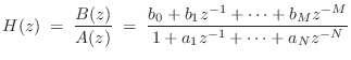
In summary, the partial fraction expansion can be used to expand any rational z transform
 |
(7.17) |
for
for
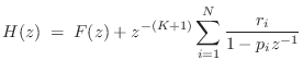
- When
 , perform a step of long division to obtain
an FIR part
, perform a step of long division to obtain
an FIR part  and a strictly proper IIR part
 .
.
- Find the
 poles
poles  ,
,
 (roots of
  ).
).
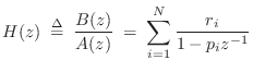
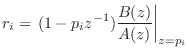
- If the poles are distinct, find the residues
 ,
from
,
from
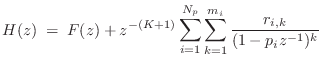
- If there are repeated poles, find the additional residues via
the method of §6.8.5, and the general form of the PFE is
where denotes the number of distinct poles, and
 denotes the multiplicity of the
  th pole.
In step 2, the poles are typically found by factoring the
denominator polynomial ![]() . This is a dangerous step numerically
which may fail when there are many poles, especially when many poles
are clustered close together in the
. This is a dangerous step numerically
which may fail when there are many poles, especially when many poles
are clustered close together in the ![]() plane.
plane.
The following matlab code illustrates factoring
![]() to
obtain the three roots,
to
obtain the three roots,
![]() ,
, ![]() :
:
A = [1 0 0 -1];  % Filter denominator polynomial
poles = roots(A) % Filter poles
See Chapter 9 for additional discussion regarding digital filters implemented as parallel sections (especially §9.2.2).
Next Section:
Software for Partial Fraction Expansion
Previous Section:
Alternate Stability Criterion


