Analytic Signals and Hilbert Transform Filters

A signal which has no negative-frequency components is called an analytic signal.^4.12 Therefore, in continuous time, every analytic signal can be represented as

$\displaystyle z(t) = \frac{1}{2\pi}\int_0^{\infty} Z(\omega)e^{j\omega t}d\omega$

where $Z(\omega)$ is the complex coefficient (setting the amplitude and phase) of the positive-frequency complex sinusoid $\exp(j\omega t)$ at frequency $\omega$ .

Any real sinusoid $A\cos(\omega t + \phi)$ may be converted to a positive-frequency complex sinusoid $A\exp[j(\omega t + \phi)]$ by simply generating a phase-quadrature component $A\sin(\omega t + \phi)$ to serve as the ``imaginary part'':

$\displaystyle A e^{j(\omega t + \phi)} = A\cos(\omega t + \phi) + j A\sin(\omega t + \phi)$

The phase-quadrature component can be generated from the in-phase component by a simple quarter-cycle time shift.^4.13

For more complicated signals which are expressible as a sum of many sinusoids, a filter can be constructed which shifts each sinusoidal component by a quarter cycle. This is called a Hilbert transform filter. Let ${\cal H}_t\{x\}$ denote the output at time of the Hilbert-transform filter applied to the signal . Ideally, this filter has magnitude at all frequencies and introduces a phase shift of $-\pi/2$ at each positive frequency and $+\pi/2$ at each negative frequency. When a real signal and its Hilbert transform $y(t) = {\cal H}_t\{x\}$ are used to form a new complex signal , the signal is the (complex) analytic signal corresponding to the real signal . In other words, for any real signal , the corresponding analytic signal $z(t)=x(t) + j {\cal H}_t\{x\}$ has the property that all ``negative frequencies'' of have been ``filtered out.''

To see how this works, recall that these phase shifts can be impressed on a complex sinusoid by multiplying it by $\exp(\pm j\pi/2) = \pm j$ . Consider the positive and negative frequency components at the particular frequency $\omega_0$ :

$\begin{eqnarray*} x_+(t) &\isdef & e^{j\omega_0 t} \\ x_-(t) &\isdef & e^{-j\omega_0 t} \end{eqnarray*}$

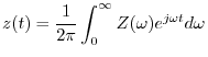
Now let's apply a degrees phase shift to the positive-frequency component, and a degrees phase shift to the negative-frequency component:

$\begin{eqnarray*} y_+(t) &=& e^{-j\pi/2} e^{j\omega_0 t} = -j e^{j\omega_0 t} \\ y_-(t) &=& e^{j\pi/2} e^{-j\omega_0 t} = j e^{-j\omega_0 t} \end{eqnarray*}$

Adding them together gives

$\begin{eqnarray*} z_+(t) &\isdef & x_+(t) + j y_+(t) = e^{j\omega_0 t} - j^2 e^{... ... x_-(t) + j y_-(t) = e^{-j\omega_0 t} + j^2 e^{-j\omega_0 t} = 0 \end{eqnarray*}$

and sure enough, the negative frequency component is filtered out. (There is also a gain of 2 at positive frequencies which we can remove by defining the Hilbert transform filter to have magnitude 1/2 at all frequencies.)

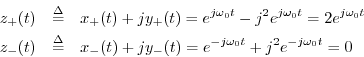
For a concrete example, let's start with the real sinusoid

$\displaystyle x(t)=2\cos(\omega_0 t) = e^{j\omega_0 t} + e^{-j\omega_0 t}.$

Applying the ideal phase shifts, the Hilbert transform is

$\begin{eqnarray*} y(t) &=& e^{j\omega_0 t-j\pi/2} + e^{-j\omega_0 t + j\pi/2}\\ &=& -je^{j\omega_0 t} + je^{-j\omega_0 t} = 2\sin(\omega_0 t). \end{eqnarray*}$

The analytic signal is then

$\displaystyle z(t) = x(t) + j y(t) = 2\cos(\omega_0 t) + j 2\sin(\omega_0 t) = 2 e^{j\omega_0 t},$

by Euler's identity. Thus, in the sum

, the negative-frequency components of

and

cancel out, leaving only the positive-frequency component. This happens for any real signal

, not just for sinusoids as in our example.

**Figure 4.16:** Creation of the analytic signal $z(t)=e^{j\omega _0 t}$ from the real sinusoid $x(t) = \cos(\omega_0 t)$ and the derived phase-quadrature sinusoid $y(t) = \sin(\omega_0 t)$ , viewed in the frequency domain. a) Spectrum of . b) Spectrum of . c) Spectrum of . d) Spectrum of .
$\includegraphics[width=2.8in]{eps/sineFD}$

Figure 4.16 illustrates what is going on in the frequency domain. At the top is a graph of the spectrum of the sinusoid $\cos(\omega_0 t)$ consisting of impulses at frequencies $\omega=\pm\omega_0$ and zero at all other frequencies (since $\cos(\omega_0 t) = (1/2)\exp(j\omega_0 t) + (1/2)\exp(-j\omega_0 t)$ ). Each impulse amplitude is equal to . (The amplitude of an impulse is its algebraic area.) Similarly, since $\sin(\omega_0 t) = (1/2j)\exp(j\omega_0 t) - (1/2j)\exp(-j\omega_0 t) = -(j/2) \exp(j\omega_0 t) + (j/2)\exp(-j\omega_0 t)$ , the spectrum of $\sin(\omega_0 t)$ is an impulse of amplitude at $\omega=\omega_0$ and amplitude at $\omega=-\omega_0$ . Multiplying by results in $j\sin(\omega_0 t) = (1/2)\exp(j\omega_0 t) - (1/2)\exp(-j\omega_0 t)$ which is shown in the third plot, Fig.4.16c. Finally, adding together the first and third plots, corresponding to , we see that the two positive-frequency impulses add in phase to give a unit impulse (corresponding to $\exp(j\omega_0 t)$ ), and at frequency $-\omega_0$ , the two impulses, having opposite sign, cancel in the sum, thus creating an analytic signal , as shown in Fig.4.16d. This sequence of operations illustrates how the negative-frequency component $\exp(-j\omega_0 t)$ gets filtered out by summing $\cos(\omega_0 t)$ with $j\sin(\omega_0 t)$ to produce the analytic signal $\exp(j\omega_0 t)$ corresponding to the real signal $\cos(\omega_0 t)$ .

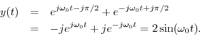
As a final example (and application), let $x(t) = A(t)\cos(\omega t)$ , where is a slowly varying amplitude envelope (slow compared with $\omega$ ). This is an example of amplitude modulation applied to a sinusoid at ``carrier frequency'' $\omega$ (which is where you tune your AM radio). The Hilbert transform is very close to $y(t)\approx A(t)\sin(\omega t)$ (if were constant, this would be exact), and the analytic signal is $z(t)\approx A(t)e^{j\omega t}$ . Note that AM demodulation^4.14is now nothing more than the absolute value. I.e., $A(t) = \left\vert z(t)\right\vert$ . Due to this simplicity, Hilbert transforms are sometimes used in making amplitude envelope followers for narrowband signals (i.e., signals with all energy centered about a single ``carrier'' frequency). AM demodulation is one application of a narrowband envelope follower.

Order a Hardcopy of Mathematics of the DFT

Previous: FM Spectra
Next: Generalized Complex Sinusoids

written by Julius Orion Smith III
Julius Smith's background is in electrical engineering (BS Rice 1975, PhD Stanford 1983). He is presently Professor of Music and Associate Professor (by courtesy) of Electrical Engineering at Stanford's Center for Computer Research in Music and Acoustics (CCRMA), teaching courses and pursuing research related to signal processing applied to music and audio systems. See http://ccrma.stanford.edu/~jos/ for details.

Sign in

Search Online Books

Free Online Books

Chapters

Mathematics of the DFT
    Sinusoids and Exponentials
       Complex Sinusoids
          Analytic Signals and Hilbert Transform Filters