


Proof of Euler's Identity
This chapter outlines the proof of Euler's Identity, which is an important tool for working with complex numbers. It is one of the critical elements of the DFT definition that we need to understand.
Euler's Identity
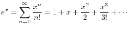
Euler's identity (or ``theorem'' or ``formula'') is
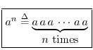
Positive Integer Exponents
The ``original'' definition of exponents which ``actually makes sense'' applies only to positive integer exponents:
Generalizing this definition involves first noting its abstract mathematical properties, and then making sure these properties are preserved in the generalization.
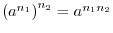
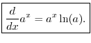
Properties of Exponents
From the basic definition of positive integer exponents, we have
- (1)
-

- (2)
-
The Exponent Zero
How should we define ![]() in a manner consistent with the
properties of integer exponents? Multiplying it by
in a manner consistent with the
properties of integer exponents? Multiplying it by ![]() gives
gives
Negative Exponents
What should ![]() be? Multiplying it by
be? Multiplying it by ![]() gives, using property (1),
gives, using property (1),


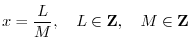
Rational Exponents
A rational number is a real number that can be expressed as a ratio of two finite integers:
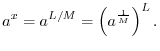
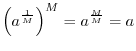
![$\displaystyle \zbox {a^{\frac{1}{M}} \isdef \sqrt[M]{a}.}
$](http://www.dsprelated.com/josimages_new/mdft/img250.png)
Real Exponents
The closest we can actually get to most real numbers is to compute a
rational number that is as close as we need. It can be shown that
rational numbers are dense in the real numbers; that is,
between every two real numbers there is a rational number, and between
every two rational numbers is a real number.3.1An irrational number can be defined as any real
number having a non-repeating decimal expansion. For example,
![]() is an irrational real number whose decimal expansion starts
out as3.2
is an irrational real number whose decimal expansion starts
out as3.2
![\begin{eqnarray*}
x &=& 0.\overline{123} \\ [5pt]
\quad\Rightarrow\quad 1000x &=...
...999x &=& 123\\ [5pt]
\quad\Rightarrow\quad x &=& \frac{123}{999}
\end{eqnarray*}](http://www.dsprelated.com/josimages_new/mdft/img261.png)
Other examples of irrational numbers include
Their decimal expansions do not repeat.
Let
![]() denote the
denote the ![]() -digit decimal expansion of an arbitrary real
number
-digit decimal expansion of an arbitrary real
number ![]() . Then
. Then
![]() is a rational number (some integer over
is a rational number (some integer over ![]() ).
We can say
).
We can say
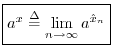
Since
![]() is defined for all
is defined for all ![]() , we naturally define
, we naturally define ![]() as the following mathematical limit:
as the following mathematical limit:
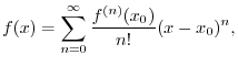
A First Look at Taylor Series
Most ``smooth'' functions ![]() can be expanded in the form of a
Taylor series expansion:
can be expanded in the form of a
Taylor series expansion:

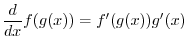
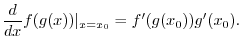
Imaginary Exponents
We may define imaginary exponents the same way that all
sufficiently smooth real-valued functions of a real variable are
generalized to the complex case--using Taylor series. A
Taylor series expansion is just a polynomial (possibly of infinitely
high order), and polynomials involve only addition, multiplication,
and division. Since these elementary operations are also defined for
complex numbers, any smooth function of a real variable ![]() may be
generalized to a function of a complex variable
may be
generalized to a function of a complex variable ![]() by simply
substituting the complex variable
by simply
substituting the complex variable ![]() for the real variable
for the real variable ![]() in the Taylor series expansion of
in the Taylor series expansion of ![]() .
.
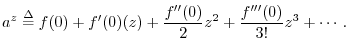
Let
![]() , where
, where ![]() is any positive real number and
is any positive real number and ![]() is
real. The Taylor
series expansion about
is
real. The Taylor
series expansion about ![]() (``Maclaurin series''),
generalized to the complex case is then
(``Maclaurin series''),
generalized to the complex case is then
This is well defined, provided the series converges for every finite
Derivatives of f(x)=a^x
Let's apply the definition of differentiation and see what happens:
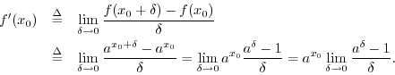
Since the limit of
![]() as
as
![]() is less than
1 for
is less than
1 for ![]() and greater than
and greater than ![]() for
for ![]() (as one can show via direct
calculations), and since
(as one can show via direct
calculations), and since
![]() is a continuous
function of
is a continuous
function of ![]() for
for ![]() , it follows that there exists a
positive real number we'll call
, it follows that there exists a
positive real number we'll call ![]() such that for
such that for ![]() we get
we get
So far we have proved that the derivative of ![]() is
is ![]() .
What about
.
What about ![]() for other values of
for other values of ![]() ? The trick is to write it as
? The trick is to write it as
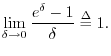
Back to e
Above, we defined ![]() as the particular real number satisfying
as the particular real number satisfying
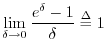
or
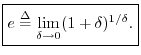
Numerically, ![]() is a transcendental number (a type of irrational
number3.5), so its decimal expansion never repeats.
The initial decimal expansion of
is a transcendental number (a type of irrational
number3.5), so its decimal expansion never repeats.
The initial decimal expansion of ![]() is given by3.6
is given by3.6
e^(j theta)
We've now defined ![]() for any positive real number
for any positive real number ![]() and any
complex number
and any
complex number ![]() . Setting
. Setting ![]() and
and ![]() gives us the
special case we need for Euler's identity. Since
gives us the
special case we need for Euler's identity. Since ![]() is its own
derivative, the Taylor series expansion for
is its own
derivative, the Taylor series expansion for ![]() is one of
the simplest imaginable infinite series:
is one of
the simplest imaginable infinite series:
Comparing the Maclaurin expansion for
![]() with that of
with that of
![]() and
and
![]() proves Euler's identity. Recall
from introductory calculus that
proves Euler's identity. Recall
from introductory calculus that
![\begin{eqnarray*}
\frac{d}{d\theta}\cos(\theta) &=& -\sin(\theta) \\ [5pt]
\frac{d}{d\theta}\sin(\theta) &=& \cos(\theta)
\end{eqnarray*}](http://www.dsprelated.com/josimages_new/mdft/img321.png)
so that
![\begin{eqnarray*}
\left.\frac{d^n}{d\theta^n}\cos(\theta)\right\vert _{\theta=0}...
...} \\ [5pt]
0, & n\;\mbox{\small even}. \\
\end{array} \right.
\end{eqnarray*}](http://www.dsprelated.com/josimages_new/mdft/img322.png)
Plugging into the general Maclaurin series gives
Separating the Maclaurin expansion for
![]() into its even and odd
terms (real and imaginary parts) gives
into its even and odd
terms (real and imaginary parts) gives
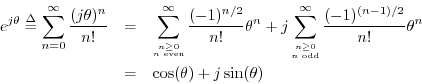
thus proving Euler's identity.
Back to Mth Roots
As mentioned in §3.4, there are ![]() different numbers
different numbers ![]() which satisfy
which satisfy ![]() when
when ![]() is a positive integer.
That is, the
is a positive integer.
That is, the ![]() th root of
th root of ![]() , which is
written as
, which is
written as ![]() , is not unique--there are
, is not unique--there are ![]() of them. How do
we find them all? The answer is to consider complex numbers in
polar form.
By Euler's Identity, which we just proved, any number,
real or complex, can be written in polar form as
of them. How do
we find them all? The answer is to consider complex numbers in
polar form.
By Euler's Identity, which we just proved, any number,
real or complex, can be written in polar form as
Roots of Unity
Since
![]() for every integer
for every integer ![]() ,
we
can write
,
we
can write
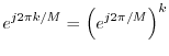
We will learn later that the ![]() th roots of unity are used to generate
all the sinusoids used by the length-
th roots of unity are used to generate
all the sinusoids used by the length-![]() DFT and its inverse.
The
DFT and its inverse.
The ![]() th complex sinusoid used in a DFT of length
th complex sinusoid used in a DFT of length ![]() is given by
is given by
Direct Proof of De Moivre's Theorem
In §2.10, De Moivre's theorem was introduced as a consequence of Euler's identity:
Proof:
To establish the ``basis'' of our mathematical induction proof, we may
simply observe that De Moivre's theorem is trivially true for
![]() . Now assume that De Moivre's theorem is true for some positive
integer
. Now assume that De Moivre's theorem is true for some positive
integer ![]() . Then we must show that this implies it is also true for
. Then we must show that this implies it is also true for
![]() , i.e.,
, i.e.,
Since it is true by hypothesis that
From trigonometry, we have the following sum-of-angle identities:
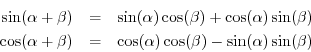
These identities can be proved using only arguments from classical
geometry.3.8Applying these to the right-hand side of Eq.![]() (3.3), with
(3.3), with
![]() and
and
![]() , gives Eq.
, gives Eq.![]() (3.2), and
so the induction step is proved.
(3.2), and
so the induction step is proved.
![]()
De Moivre's theorem establishes that integer powers of
![]() lie on a circle of radius 1 (since
lie on a circle of radius 1 (since
![]() , for all
, for all
![]() ). It
therefore can be used to determine all
). It
therefore can be used to determine all ![]() of the
of the ![]() th roots of unity
(see §3.12 above).
However, no definition of
th roots of unity
(see §3.12 above).
However, no definition of ![]() emerges readily from De Moivre's
theorem, nor does it establish a definition for imaginary exponents
(which we defined using Taylor series expansion in §3.7 above).
emerges readily from De Moivre's
theorem, nor does it establish a definition for imaginary exponents
(which we defined using Taylor series expansion in §3.7 above).
Euler_Identity Problems
See http://ccrma.stanford.edu/~jos/mdftp/Euler_Identity_Problems.html
Next Section:
Sinusoids and Exponentials
Previous Section:
Complex Numbers


