


Matrices
A matrix is defined as a rectangular array of numbers, e.g.,
![$\displaystyle \mathbf{A}= \left[\begin{array}{cc} a & b \\ [2pt] c & d \end{array}\right]
$](http://www.dsprelated.com/josimages_new/mdft/img2046.png)
![$\displaystyle \left[\begin{array}{cc} a & b \\ c & d \\ e & f \end{array}\right].
$](http://www.dsprelated.com/josimages_new/mdft/img2050.png)
The transpose of a real matrix
![]() is denoted by
is denoted by
![]() and is defined by
and is defined by
![$\displaystyle \left[\begin{array}{cc} a & b \\ c & d \\ e & f \end{array}\right...
...\tiny T}}
=\left[\begin{array}{ccc} a & c & e \\ b & d & f \end{array}\right].
$](http://www.dsprelated.com/josimages_new/mdft/img2064.png)
A complex matrix
![]() , is simply a
matrix containing complex numbers. The
transpose of a complex matrix is normally defined to
include conjugation. The conjugating transpose operation is called the
Hermitian transpose. To avoid confusion, in this tutorial,
, is simply a
matrix containing complex numbers. The
transpose of a complex matrix is normally defined to
include conjugation. The conjugating transpose operation is called the
Hermitian transpose. To avoid confusion, in this tutorial,
![]() and the word ``transpose'' will always denote transposition
without conjugation, while conjugating transposition will be
denoted by
and the word ``transpose'' will always denote transposition
without conjugation, while conjugating transposition will be
denoted by ![]() and be called the ``Hermitian transpose'' or the
``conjugate transpose.'' Thus,
and be called the ``Hermitian transpose'' or the
``conjugate transpose.'' Thus,
Matrix Multiplication
Let
![]() be a general
be a general ![]() matrix and let
matrix and let
![]() denote a
general
denote a
general ![]() matrix. Denote the matrix product by
matrix. Denote the matrix product by
![]() . Then matrix multiplication is carried out by computing
the inner product of every row of
. Then matrix multiplication is carried out by computing
the inner product of every row of
![]() with every column of
with every column of
![]() . Let the
. Let the ![]() th row of
th row of
![]() be denoted by
be denoted by
![]() ,
,
![]() , and the
, and the ![]() th column of
th column of
![]() by
by
![]() ,
,
![]() . Then the matrix product
. Then the matrix product
![]() is
defined as
is
defined as
![$\displaystyle \mathbf{C}= \mathbf{A}^{\!\hbox{\tiny T}}\, \mathbf{B}= \left[\be...
...cdots & <\underline{a}^{\hbox{\tiny T}}_M,\underline{b}_N>
\end{array}\right].
$](http://www.dsprelated.com/josimages_new/mdft/img2081.png)
Examples:
![$\displaystyle \left[\begin{array}{cc} a & b \\ c & d \\ e & f \end{array}\right...
...gamma & c\beta+d\delta \\
e\alpha+f\gamma & e\beta+f\delta
\end{array}\right]
$](http://www.dsprelated.com/josimages_new/mdft/img2084.png)
![$\displaystyle \left[\begin{array}{cc} \alpha & \beta \\ \gamma & \delta \end{ar...
...ma a + \delta b & \gamma c + \delta d & \gamma e + \delta f
\end{array}\right]
$](http://www.dsprelated.com/josimages_new/mdft/img2085.png)
![$\displaystyle \left[\begin{array}{c} \alpha \\ \beta \end{array}\right]
\cdot
\...
...pha a & \alpha b & \alpha c \\
\beta a & \beta b & \beta c
\end{array}\right]
$](http://www.dsprelated.com/josimages_new/mdft/img2086.png)
![$\displaystyle \left[\begin{array}{ccc} a & b & c \end{array}\right]
\cdot
\left...
...} \alpha \\ \beta \\ \gamma \end{array}\right]
= a \alpha + b \beta + c \gamma
$](http://www.dsprelated.com/josimages_new/mdft/img2087.png)
An ![]() matrix
matrix
![]() can be multiplied on the right by an
can be multiplied on the right by an
![]() matrix, where
matrix, where ![]() is any positive integer. An
is any positive integer. An ![]() matrix
matrix
![]() can be multiplied on the left by a
can be multiplied on the left by a ![]() matrix, where
matrix, where ![]() is any positive integer. Thus, the number of columns in
the matrix on the left must equal the number of rows in the matrix on the
right.
is any positive integer. Thus, the number of columns in
the matrix on the left must equal the number of rows in the matrix on the
right.
Matrix multiplication is non-commutative, in general. That is,
normally
![]() even when both products are defined (such as when the
matrices are square.)
even when both products are defined (such as when the
matrices are square.)
The transpose of a matrix product is the product of the transposes in reverse order:
The identity matrix is denoted by
![]() and is defined as
and is defined as
![$\displaystyle \mathbf{I}\isdef \left[\begin{array}{ccccc}
1 & 0 & 0 & \cdots &...
...dots & \vdots & \cdots & \vdots \\
0 & 0 & 0 & \cdots & 1
\end{array}\right]
$](http://www.dsprelated.com/josimages_new/mdft/img2091.png)
As a special case, a matrix
![]() times a vector
times a vector
![]() produces a new vector
produces a new vector
![]() which consists of the inner product of every row of
which consists of the inner product of every row of
![]() with
with
![]()
![$\displaystyle \mathbf{A}^{\!\hbox{\tiny T}}\underline{x}= \left[\begin{array}{c...
...vdots \\
<\underline{a}^{\hbox{\tiny T}}_M,\underline{x}>
\end{array}\right].
$](http://www.dsprelated.com/josimages_new/mdft/img2097.png)
As a further special case, a row vector on the left may be multiplied by a column vector on the right to form a single inner product:
Solving Linear Equations Using Matrices
Consider the linear system of equations
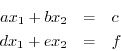
in matrix form:
![$\displaystyle \left[\begin{array}{cc} a & b \\ [2pt] d & e \end{array}\right] \...
..._2 \end{array}\right] = \left[\begin{array}{c} c \\ [2pt] f \end{array}\right]
$](http://www.dsprelated.com/josimages_new/mdft/img2101.png)
![$\displaystyle \underline{x}= \mathbf{A}^{-1}\underline{b}= \left[\begin{array}{...
...\end{array}\right]^{-1}\left[\begin{array}{c} c \\ [2pt] f \end{array}\right].
$](http://www.dsprelated.com/josimages_new/mdft/img2104.png)
![$\displaystyle \left[\begin{array}{cc} a & b \\ [2pt] d & e \end{array}\right]^{...
...rac{1}{ae-bd}\left[\begin{array}{cc} e & -b \\ [2pt] -d & a \end{array}\right]
$](http://www.dsprelated.com/josimages_new/mdft/img2105.png)
Next Section:
Matlab/Octave Examples
Previous Section:
Number Systems for Digital Audio


