


Spectral Phase
As for the phase of the spectrum, what do we expect? We have chosen
the sinusoid phase offset to be zero. The window is causal and
symmetric about its middle. Therefore, we expect a linear phase term
with slope
![]() samples (as discussed in connection with the
shift theorem in §7.4.4).
Also, the window transform has sidelobes which cause a phase of
samples (as discussed in connection with the
shift theorem in §7.4.4).
Also, the window transform has sidelobes which cause a phase of ![]() radians to switch in and out. Thus, we expect to see samples of a
straight line (with slope
radians to switch in and out. Thus, we expect to see samples of a
straight line (with slope ![]() samples) across the main lobe of the
window transform, together with a switching offset by
samples) across the main lobe of the
window transform, together with a switching offset by ![]() in every
other sidelobe away from the main lobe, starting with the immediately
adjacent sidelobes.
in every
other sidelobe away from the main lobe, starting with the immediately
adjacent sidelobes.
In Fig.8.9(a), we can see the negatively sloped line
across the main lobe of the window transform, but the sidelobes are
hard to follow. Even the unwrapped phase in Fig.8.9(b)
is not as clear as it could be. This is because a phase jump of ![]() radians and
radians and ![]() radians are equally valid, as is any odd multiple
of
radians are equally valid, as is any odd multiple
of ![]() radians. In the case of the unwrapped phase, all phase jumps
are by
radians. In the case of the unwrapped phase, all phase jumps
are by ![]() starting near frequency
starting near frequency ![]() .
Figure 8.9(c) shows what could be
considered the ``canonical'' unwrapped phase for this example: We see
a linear phase segment across the main lobe as before, and outside the
main lobe, we have a continuation of that linear phase across all of
the positive sidelobes, and only a
.
Figure 8.9(c) shows what could be
considered the ``canonical'' unwrapped phase for this example: We see
a linear phase segment across the main lobe as before, and outside the
main lobe, we have a continuation of that linear phase across all of
the positive sidelobes, and only a ![]() -radian deviation from that
linear phase across the negative sidelobes. In other words, we see a
straight linear phase at the desired slope interrupted by temporary
jumps of
-radian deviation from that
linear phase across the negative sidelobes. In other words, we see a
straight linear phase at the desired slope interrupted by temporary
jumps of ![]() radians. To obtain unwrapped phase of this type, the
unwrap function needs to alternate the sign of successive
phase-jumps by
radians. To obtain unwrapped phase of this type, the
unwrap function needs to alternate the sign of successive
phase-jumps by ![]() radians; this could be implemented, for example,
by detecting jumps-by-
radians; this could be implemented, for example,
by detecting jumps-by-![]() to within some numerical tolerance and
using a bit of state to enforce alternation of
to within some numerical tolerance and
using a bit of state to enforce alternation of ![]() with
with ![]() .
.
To convert the expected phase slope from ![]() ``radians per
(rad/sec)'' to ``radians per cycle-per-sample,'' we need to multiply
by ``radians per cycle,'' or
``radians per
(rad/sec)'' to ``radians per cycle-per-sample,'' we need to multiply
by ``radians per cycle,'' or ![]() . Thus, in
Fig.8.9(c), we expect a slope of
. Thus, in
Fig.8.9(c), we expect a slope of ![]() radians
per unit normalized frequency, or
radians
per unit normalized frequency, or ![]() radians per
radians per ![]() cycles-per-sample, and this looks about right, judging from the plot.
cycles-per-sample, and this looks about right, judging from the plot.

Raw spectral phase and its interpolation 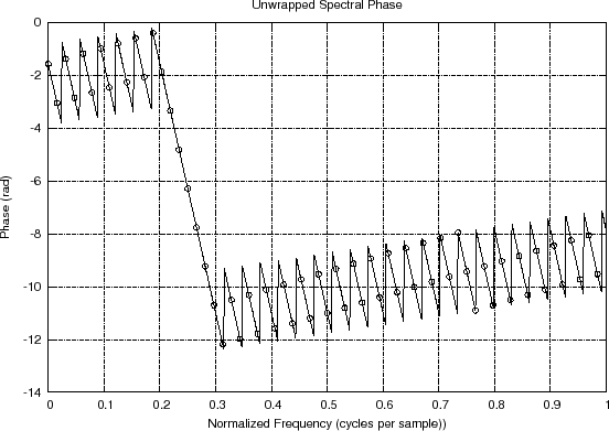
Unwrapped spectral phase and its interpolation 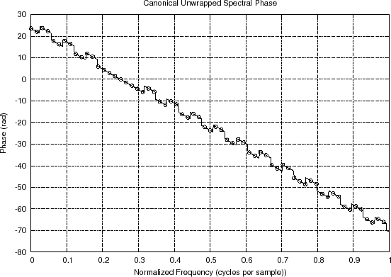
Canonically unwrapped spectral phase and its interpolation |
Next Section:
Radix 2 FFT Complexity is N Log N
Previous Section:
Hann Window Spectrum Analysis Results


