


Example: FIR-Filtered White Noise
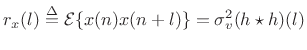
Let's estimate the autocorrelation and power spectral density of the ``moving average'' (MA) process
| (7.34) |
where
Since
![]() ,
,
| (7.35) |
for nonnegative lags (
![$\displaystyle (h\star h)(l) = \left\{\begin{array}{ll} 8-l, & \vert l\vert<8 \\ [5pt] 0, & \vert l\vert\ge 8. \\ \end{array} \right.$](http://www.dsprelated.com/josimages_new/sasp2/img1206.png) |
(7.36) |
Thus, the autocorrelation of
 |
(7.37) |
The true power spectral density (PSD) is then
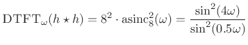 |
(7.38) |
Figure 6.3 shows a collection of measured autocorrelations together with their associated smoothed-PSD estimates.
![\includegraphics[width=\twidth]{eps/tcolored}](http://www.dsprelated.com/josimages_new/sasp2/img1209.png) |
Next Section:
Example: Synthesis of 1/F Noise (Pink Noise)
Previous Section:
Matlab for Welch's Method


