Compute the Frequency Response of a Multistage Decimator

• Matlab
• Multirate DSP
• Tutorials

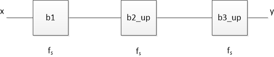
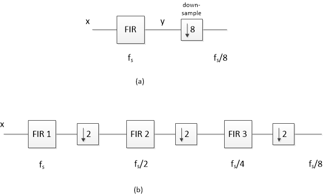
Figure 1a shows the block diagram of a decimation-by-8 filter, consisting of a low-pass finite impulse response (FIR) filter followed by downsampling by 8 [1].  A more efficient version is shown in Figure 1b, which uses three cascaded decimate-by-two filters.  This implementation has the advantages that only FIR 1 is sampled at the highest sample rate, and the total number of filter taps is lower.

The frequency response of the single-stage decimator before downsampling is just the response of the FIR filter from f = 0 to f_s/2.  After downsampling, remaining signal components above f_s/16 create aliases at frequencies below f_s/16.  It’s not quite so clear how to find the frequency response of the multistage filter:  after all, the output of FIR 3 has unique spectrum extending only to f_s/8, and we need to find the response from 0 to f_s/2.  Let’s look at an example to see how to calculate the frequency response.  Although the example uses decimation-by-2 stages, our approach applies to any integer decimation factor.

This article is available in PDF format for easy printing.

Figure 1.  Decimation by 8.  (a)  Single-stage decimator.  (b)  Three-stage decimator.

For this example, let the input sample rate of the decimator in Figure 1b equal 1600 Hz.  The three FIR filters then have sample rates of 1600, 800, and 400 Hz.  Each is a half-band filter [2 - 4] with passband of at least 0 to 75 Hz.  Here is Matlab code that defines the three sets of filter coefficients (See Appendix):

    b1= [-1 0 9 16 9 0 -1]/32;                            % fs = 1600 Hz
    b2= [23 0 -124 0 613 1023 613 0 -124 0 23]/2048;      % fs/2 = 800 Hz
    b3= [-11 0 34 0 -81 0 173 0 -376 0 1285 2050 1285 0 -376 0 173 0 ...
         -81 0 34 0 -11]/4096;                            % fs/4 = 400 Hz

The frequency responses of these filters are plotted in Figure 2.  Each response is plotted over f = 0 to half its sampling rate:

FIR 1:  0 to 800 Hz

FIR 2:  0 to 400 Hz

FIR 3:  0 to 200 Hz

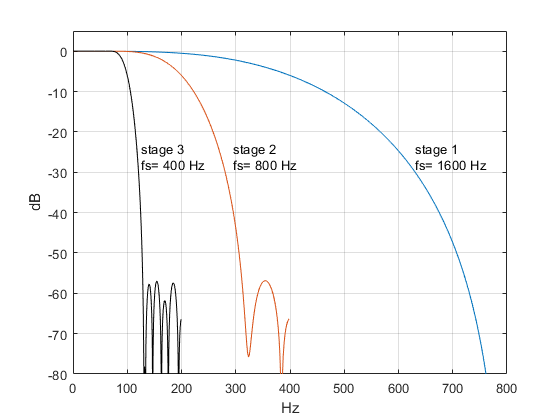
Figure 2.  Frequency Responses of halfband decimation filters.              

Now, to find the overall response at f_s = 1600 Hz, we need to know the time or frequency response of FIR 2 and FIR 3 at this sample rate.  Converting the time response is just a matter of sampling at f_s instead of at  f_s /2 or f_s /4 – i.e., upsampling.  For example, the following Matlab code upsamples the FIR 2 coefficients by 2, from f_s/2 to f_s:

    b2_up= zeros(1,21);
    b2_up(1:2:21)= b2;

Figure 3 shows the coefficients b2 and b2_up.  The code has inserted samples of value zero halfway between each of the original samples of b2 to create b2_up.  b2_up now has a sample rate of f_s.  But although we have a new representation of the coefficients, upsampling has no effect on the math:  b2_up and b2 have the same coefficient values and the same time interval between the coefficients.

For FIR 3, we need to upsample by 4 as follows:

    b3_up= zeros(1,89);
    b3_up(1:4:89)= b3;

Figure 4 shows the coefficients b3 and b3_up.  Again, the upsampled version is mathematically identical to the original version.  Now we have three sets of coefficients, all sampled at f_s = 1600 Hz.  A block diagram of the cascade of these coefficients is shown in Figure 5.

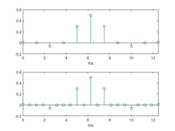
Figure 3.  Top:  Halfband filter coefficients b2.    Bottom:  Coefficients upsampled by 2.      

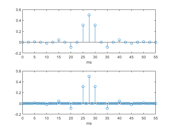
Figure 4.  Top:  Halfband filter coefficients b3.    Bottom:  Coefficients upsampled by 4.        

Using the DFT, we can compute and plot the frequency response of each filter stage, as shown in Figure 6.  Upsampling b2 and b3 has allowed us to compute the DFT at the input sampling frequency f_s for those sections.  The sampling theorem [5] tells us that the frequency response of b2, which has a sample rate of 800 Hz, has an image between 400 and 800 Hz.  Since b2_up has a sample rate of 1600 Hz, this image appears in its DFT (middle plot).  Similarly, the DFT of b3_up has images from 200 to 400; 400 to 600; and 600 to 800 Hz (bottom plot).

Each decimation filter response in Figure 6 has stopband centered at one-half of its original sample frequency, shown as a red horizontal line (see Appendix).  This attenuates spectrum in that band prior to downsampling by 2.

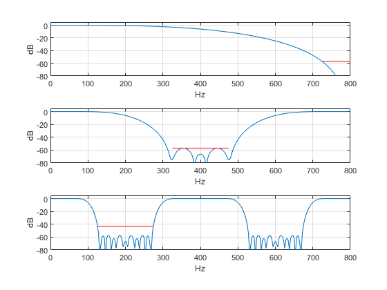
Figure 6.   Frequency responses of decimator stages, f_s = 1600 Hz.                  

Top:  FIR 1 (b1 )    Middle:  FIR 2 (b2_up)    Bottom:  FIR 3 (b3_up)             

Now let’s find the overall frequency response.  To do this, we could a) find the product of the three frequency responses in Figure 6, or b) compute the impulse response of the cascade of b1, b2_up, and b3_up, then use it to find H(z).  Taking the latter approach, the overall impulse response is:

b₁₂₃ = b₁ ⊛ (b_2up ⊛ b_3up)

where ⊛ indicates convolution.  The Matlab code is:

    b23= conv(b2_up,b3_up);
    b123= conv(b23,b1);        % overall impulse response at fs= 1600 Hz

The impulse response is plotted in Figure 7.  It is worth comparing the length of this response to that of the decimator stages.  The impulse response has 115 samples; that is, it would take a 115-tap FIR filter to implement the decimator as a single stage FIR sampled at 1600 Hz.  Of the 115 taps, 16 are zero.  By contrast, the length of the three decimator stages are 7, 11, and 23 taps, of which a total of 16 taps are zero.  So the multistage approach saves taps, and furthermore, only the first stage operates at 1600 Hz.  Thus, the multistage decimator uses significantly fewer resources than a single stage decimator.

Calculating the frequency response from b_123:

    fs= 1600;                    % Hz decimator input sample rate
    [h,f]= freqz(b123,1,256,fs);
    H= 20*log10(abs(h));         % overall freq response magnitude

The frequency response magnitude is plotted in Figure 8, with the stopband specified in the Appendix shown in red.

Here is a summary of the steps to compute the decimator frequency response:

1. Upsample the coefficients of all of the decimator stages (except the first stage) so that their sample rate equals the input sample rate.
2. Convolve all the coefficients from step 1 to obtain the overall impulse response at the input sample rate.
3. Take the DFT of the overall impulse response to obtain the frequency response.

Our discussion of upsampling may bring to mind the use of that process in interpolators.  As in our example, upsampling in an interpolator creates images of the signal spectrum at multiples of the original sample frequency.  The interpolation filter then attenuates those images [6].

We don’t want to forget aliasing, so we’ll take a look at that next.

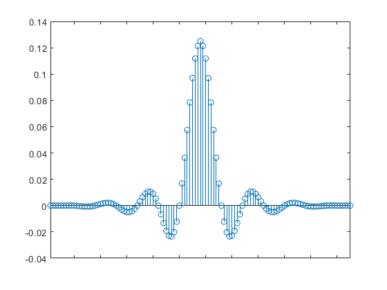
Figure 7.  Overall impulse response of three-stage decimator at f_s = 1600 Hz (length = 115).          

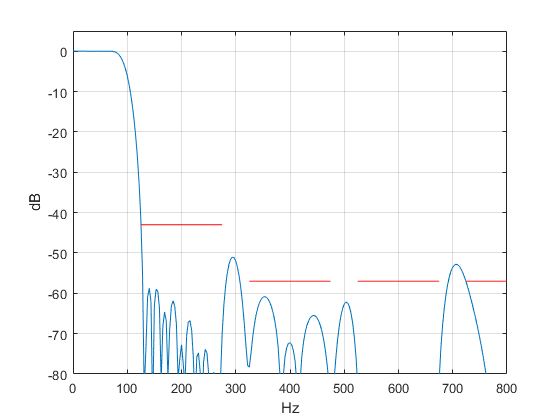
Figure 8.  Overall frequency response of Decimator at f_s= 1600 Hz.               

Taking Aliasing into Account

The output sample rate of the decimator in Figure 1b is f_{s out}  = 1600/8 = 200 Hz.  If we apply sinusoids to its input, they will be filtered by the response of Figure 8, but then any components above f_{s out} /2 (100 Hz) will produce aliases in the band of 0 to f_{s out} /2.  Let’s apply equal level sinusoids at 75, 290, and 708 Hz, as shown in Figure 9.  The response in the bottom of Figure 9 shows the expected attenuation at 290 Hz is about 52 dB and at 708 Hz is about 53 dB (red dots).  For reference, the component at 75 Hz has 0 dB attenuation.  After decimation, the components at 290 and 708 Hz alias as follows:

f₁ = 290 – f_{s out}  = 290 – 200 = 90 Hz

f₂ = 4*f_{s out}  – 708 = 800 – 708 = 92 Hz

So, after decimation, we expect a component at 90 MHz that is about 52 dB below the component at 75 Hz, and a component at 92 Hz that is about 53 dB down.  This is in fact what we get when we go through the filtering and downsampling operations:  see Figure 10.

Note that the sines at 290 and 708 MHz are not within the stopbands as defined in the Appendix for FIR 1 and FIR 2.  For that reason, the aliased components are greater than the specified stopband of -57 dB.  This is not necessarily a problem, however, because they fall outside the passband of 75 Hz.  They can be further attenuated by a subsequent channel filter.

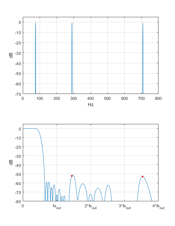
Figure 9.  Top:  Multiple sinusoidal input to decimator at 75, 290, and 708 Hz.            

Bottom:  Decimator overall frequency response.  Note f_{s out} = f_s/8.  

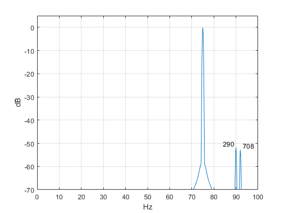
Figure 10.  Decimator output spectrum for input of Figure 9.  f_{s out} = f_s/8 = 200 Hz.          

Appendix:  Decimation Filter Synthesis

The halfband decimators were designed by the window method [3] using Matlab function fir1.  We obtain halfband coefficients by setting the cutoff frequency to one-quarter of the sample rate.  The order of each filter was chosen to meet the passband and stopband requirements shown in the table.  Frequency responses are plotted in Figure 2 of the main text.  We could have made the stopband attenuation of FIR 3 equal to that of the other filters, at the expense of more taps.

Common parameters:

Passband:  > -0.1 dB at 75 Hz

Window function:  Chebyshev, -47 dB

Note that the filters as synthesized by fir1 have zero-valued coefficients on each end, so the actual filter order is two less than that in the function call.  Using N = 6 and 10 in fir1 (instead of 8 and 12) would eliminate these superfluous zero coefficients, but would result in somewhat different responses.

% dec_fil1.m    1/31/19 Neil Robertson
% synthesize halfband decimators using window method
% fc = (fs/4)/fnyq = (fs/4)/(fs/2) = 1/2
% resulting coeffs have zeros on the each end,so actual filter order is N-2.
%
> fc= 1/2;      % -6 dB freq divided by nyquist freq
%
% b1: halfband decimator from fs= 1600 Hz to 800 Hz
N= 8;
win= chebwin(N+1,47);         % chebyshev window function, -47 dB
b= fir1(N,fc,win);            % filter synthesis by window method
b1= round(b*32)/32;           % fixed-point coefficients
%
% b2: halfband decimator from fs= 800 Hz to 400 Hz
N= 12;
win= chebwin(N+1,47);
b= fir1(N,fc,win);
b2= round(b*2048)/2048;
%
% b3: halfband decimator from fs= 400 Hz to 200 Hz
N= 24;
win= chebwin(N+1,47);
b= fir1(N,fc,win);
b3= round(b*4096)/4096;

References

1.  Lyons, Richard G. , Understanding Digital Signal Processing, 2^nd Ed., Prentice Hall, 2004, section 10.1.
2. Mitra, Sanjit K.,Digital Signal Processing, 2^nd Ed., McGraw-Hill, 2001, p 701-702.
3. Robertson, Neil, “Simplest Calculation of Halfband Filter Coefficients”, DSP Related website, Nov, 2017 https://www.dsprelated.com/showarticle/1113.php
4. Lyons, Rick, “Optimizing the Half-band Filters in Multistage Decimation and Interpolation”, DSP Related website, Jan, 2016 https://www.dsprelated.com/showarticle/903.php
5. Oppenheim, Alan V. and Shafer, Ronald W., Discrete-Time Signal Processing, Prentice Hall, 1989, Section 3.2.
6. Lyons, Richard G. , Understanding Digital Signal Processing, 2^nd Ed., Prentice Hall, 2004, section 10.2.

Neil Robertson       February 2019

Sign in