Second Order Discrete-Time System Demonstration

• Matlab
• Tutorials

Discrete-time systems are remarkable:  the time response can be computed from mere difference equations, and the coefficients a_i, b_i of these equations are also the coefficients of H(z).  Here, I try to illustrate this remarkableness by converting a continuous-time second-order system to an approximately equivalent discrete-time system.  With a discrete-time model, we can then easily compute the time response to any input.  But note that the goal here is as much to understand the discrete-time model as it is to find the response.

Consider a second-order continuous-time system [1,2] with the following transfer function:

$$H(s)=\frac{\omega_n^2}{s^2+2\zeta\omega_ns+\omega_n^2} \qquad(1)$$

ζ (zeta) is called the damping ratio and ω_n is called the natural frequency.  These two parameters completely define H(s).  The system has two finite poles and two zeros at ω = ∞.

The poles of H(s) are $-\zeta\omega_n \pm \omega_n\sqrt{\zeta^2-1}$ .  For 0 < ζ < 1, the system is said to be underdamped, and the poles are complex-conjugate.  For ζ > 1, the system is overdamped, and the poles are real.  For ζ = 1, the system is critically damped, and there are two real poles, both at -ω_n.  Figure 1a shows the s-plane of an underdamped system with complex-conjugate poles, and Figure 1b shows an overdamped system with real poles.  When we convert these systems to discrete-time ones, we’ll find that, for sample frequency f_s = 100 Hz, the z-plane poles are as shown in Figures 1c and 1d.

In Section 1, we’ll develop a Matlab function that converts H(s) to a discrete-time system H(z), and plots the system’s poles, impulse response, and frequency response. Then we’ll show several example system responses.  We’ll see that having a discrete-time model makes it easy to find the time response to an arbitrary input.  In section 2, we’ll compare the time and frequency responses of the discrete-time system to those of the continuous-time system.

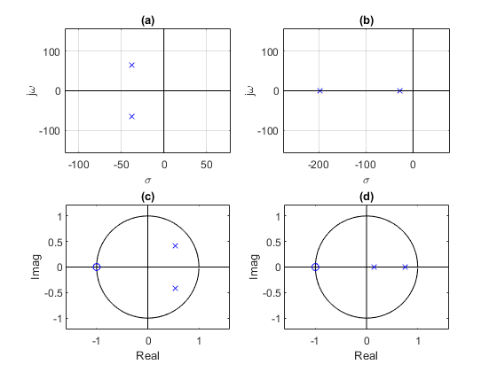
Figure 1.Second Order System Poles, ω_n = 2π*12 rad/s.

a.  s-domain, ζ = 0.5.   b.  s-domain, ζ = 1.5

c.  z-domain, ζ = 0.5, f_s= 100 Hz.    d.  z-domain, ζ = 1.5, f_s = 100 Hz.

1.  Finding the discrete-time system transfer function

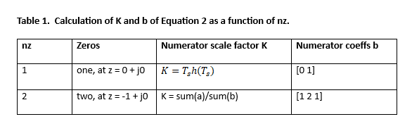
A second-order discrete-time system’s transfer function can be written as [3]:

$$H(z)= K\frac{b_0+b_1z^{-1}+b_2z^{-2}}{1+a_1z^{-1}+a_2z^{-2}} \qquad(2)$$

To find the coefficients of H(z), we’ll start by finding the pole locations in the z-plane.  The continuous time system’s poles are:

$$p_{a1}=-\zeta\omega_n+\omega_n\sqrt{\zeta^2-1}$$

$$p_{a2}=-\zeta\omega_n-\omega_n\sqrt{\zeta^2-1}$$

As already mentioned, for ζ < 1, the poles are complex-conjugate.  Using the definition of z:  z= exp(sT_s), the z-plane poles are:

$$p_1= exp(p_{a1}T_s)  \qquad \quad$$

$$p_2= exp(p_{a2}T_s) \qquad(3)$$

The denominator of H(z) is then:

$$ den=(1-p_1z^{-1})(1-p_2z^{-1}) $$

$$ =1-(p_1+p_2)z^{-1}+p_1p_2z^{-2} $$

Now consider the numerator of H(z).   As mentioned, the continuous time system has two zeros at ω = ∞.  For the discrete-time system, we have the option of using two, one, or no zeros.  Unfortunately, we cannot place zeros at ω = ∞.  The location of the zeros will affect how similar the discrete time system’s time and frequency responses are to those of the continuous time system (We’ll compare the results for two different zero locations in Section 2).  If we place a zero at z = -1 + j0, this falls on the unit circle at e^jπ.  You may recall that this point corresponds to f = f_s/2:  exp(jωT_s) = exp(j2πf_s/2 * Ts) = e^jπ.  For our initial examples, we’ll place two zeros at z = -1 + j0.  The numerator of Equation 2 becomes:

$$ num=(1+z^{-1})(1+z^{-1}) $$

$$ = 1+2z^{-1}+z^{-2} $$

So now we can list the coefficients of Equation 2:

[b₀ b₁ b₂] = [1 2 1]

[a₀ a₁ a₂] = [1 -(p₁ + p₂) p₁p₂],

where p₁ and p₂ are the z-plane poles from Equation 3.  Finally, we note that H(jω) has gain of 1 at ω = 0.  So we will choose K in Equation 2 for a gain of 1 at f = 0.  At f = 0, z = e^j0 = 1.Thus:

H(z=1) = 1 = K*sum(b)/sum(a), and

K = sum(a)/sum(b)

We now have all the equations needed to compute the coefficients of H(z), given ζ, ω_n, and f_s. The Matlab function so_demo.m is listed in the appendix of the pdf document.  Besides computing the coefficients of H(z), it plots the poles of H(s), poles and zeros of H(z), and the impulse and frequency responses of H(z).

Here is a summary of the steps we used to convert H(s) to H(z), where H(z) has the form shown in Equation 2:

1. Compute the poles p_a1 and p_a2 of H(s).
2. Convert these poles to z-plane poles p₁ and p₂.
3. Find H(z) denominator coefficients a from p₁ and p₂.
4. Assign two z-plane zeros at z = -1 + j0, giving H(z) numerator coefficients b = [1 2 1].
5. Compute K to provide gain of 1 at f = 0.

.

Example 1 – underdamped system

We’ll use so_demo.m to create a system with ζ = 0.2, f_n = 7 Hz, and f_s = 100 Hz.  The Matlab code is as follows:

    zeta= 0.2;        % damping ratio
    fn= 7;            % Hz natural frequency
    fs= 100;          % Hz sample frequency
    nz= 2;            % number of zeros
    [K,b,a]= so_demo(zeta,fn,fs,nz)

The function calculates K, b, and a as:

    K = 0.0436
    b = 1  2  1
    a = 1.0000  -1.6641  0.8387

The graphic results are plotted by so_demo.m, as shown in Figure 2.  As math dictates, the poles in the left half of the s-plane are transformed to fall inside the unit circle of the z-plane.  There are nz = 2 z-domain zeros at z = -1 + j0.  The impulse response is oscillatory with decaying amplitude – an underdamped response.  Note that if nz were equal to 1, so_demo.m would assign a single zero at z = 0 +j0 (See Section 2).

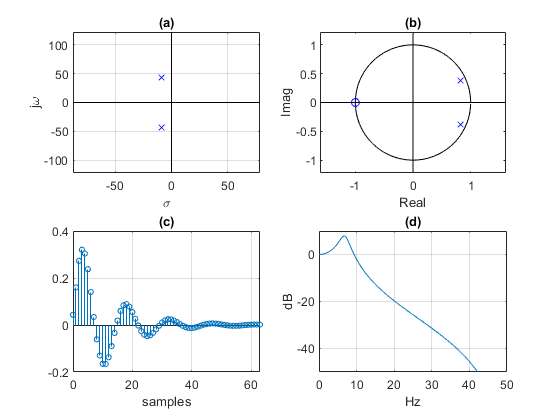
Figure 2.  Second-order system, ζ = 0.2, f_n = 7 Hz, and f_s = 100 Hz.

a.  s-domain poles.    b.  z-domain poles and zeros

c.  Impulse response.    d.  Frequency response magnitude.

Step response

We can find the response to any input simply by using the system’s difference equations, computed by the Matlab function filter [4].  The Matlab code to compute the step response is:

    N= 64;
    x= ones(1,N);            % unit step
    y= filter(K*b,a,x);      % step response

The step response is shown in Figure 3.

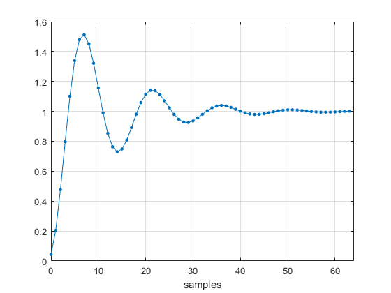
Figure 3.  Second-order system step response, ζ = 0.2, f_n = 7 Hz, and f_s = 100 Hz.

Response to a slew-rate limited step

Here, the input a signal is a slew-rate limited step that reaches its final value after 8 samples.  Here is the code to generate the input and compute the time response:

    N= 64;
    u= ones(1,N);
    v= ones(1,8)/8;
    x= conv(u,v);            % slew-rate limited pulse
    y= filter(K*b,a,x);      % response

The input signal and time response are shown in Figure 4.

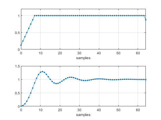
Figure 4.  Top:  Slew-rate limited step input.

Bottom:  Second-order system output, ζ = 0.2, f_n = 7 Hz, and f_s = 100 Hz.

Example 2 – overdamped system

This example again uses f_n = 7 Hz, and f_s = 100 Hz, but ζ = 1.5, resulting in an overdamped system with real poles.  See Figure 5.  The impulse response has no oscillations.

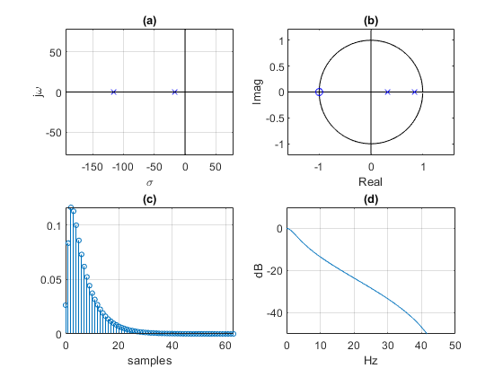
Figure 5.  Second-order system, ζ = 1.5, f_n = 7 Hz, and f_s = 100 Hz.

a.  s-domain poles.    b.  z-domain poles and zeros

c.  Impulse response.    d.  Frequency response magnitude.

Example 3 – sinusoidal impulse response

Here we let f_n = 7 Hz, and f_s = 100 Hz, with ζ = 0.  This is an unstable system with s-plane poles on the jω axis and z-plane poles on the unit circle.  Its impulse response is a sinewave at f_n (Figure 6).

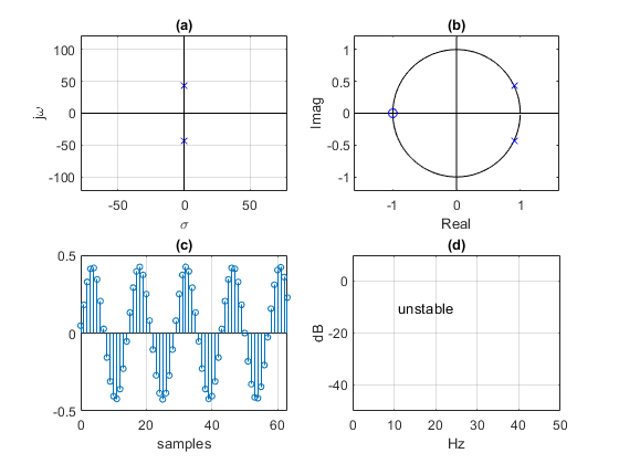
Figure 6.  Second-order system, ζ = 0, f_n = 7 Hz, and f_s = 100 Hz.

a.  s-domain poles.    b.  z-domain poles and zeros.

c.  Impulse response.    d.  Frequency response.

Example 4 – Butterworth lowpass filter

Here, f_n = 10 Hz, f_s = 100 Hz, and ζ = 1/sqrt(2) ~= 0.707.This results in s-plane poles at ω_n*(0.707 +/- 0.707).  These are the poles of a second-order Butterworth lowpass filter with -3 dB frequency of f_n Hz.  The discrete-time version has a -3 dB point that is slightly less than 10 Hz due to the zeros at f_s/2 (Figure 7).  A practical approach for designing Butterworth filters of any order uses the bilinear transform [5].

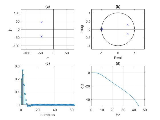
Figure 7.  Second-order system, ζ = 0.707, f_n = 10 Hz, and f_s = 100 Hz (Butterworth lowpass).

a.  s-domain poles.    b.  z-domain poles and zeros.

c.  Impulse response.    d.  Frequency response magnitude.

2.  Comparing discrete-time and continuous-time responses

Let’s consider an underdamped (ζ < 1) second-order system with H(s) given by Equation 1.  The impulse response is [2]:

$$h(t)=\frac{\omega_n}{\sqrt{1-\zeta^2}}exp(-\zeta\omega_nt) \cdot sin(\omega_n\sqrt{1-\zeta^2}\,t)\,u(t)\qquad(\zeta<1)$$

We’ll compare the impulse responses and frequency responses of the discrete and continuous-time systems for two different choices for zeros of H(z):  two zeros at z = -1 + j0, or a single zero at z = 0 + j0.  For the single-zero case, zero location and K were computed using the impulse-invariance method (see Appendix).  Reference [6] provides a second-order system example of the impulse-invariance method.  Note that for both cases that follow, we had to multiply the discrete-time impulse response by f_s to match the amplitude of the continuous-time impulse response.

Two zeros at z = -1 + j0

Figure 8 compares the impulse responses and frequency responses of the discrete-time and continuous-time systems for ζ = 0.707 (Butterworth response), f_n= 10 Hz, and f_s = 100 Hz.  You can see some mismatch of the impulse responses.  The frequency responses diverge at higher frequencies due to the discrete system’s zeros at f_s/2 = 50 Hz.  Accuracy of the discrete-time responses can be improved by increasing the sample rate:  here, for example, we could double f_s to 200 Hz.

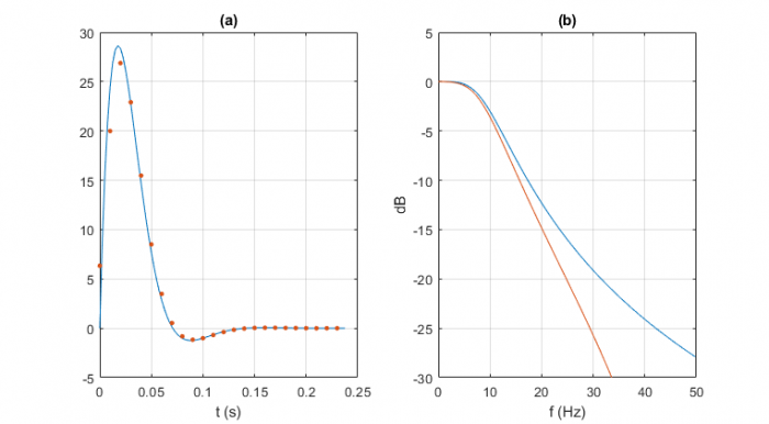
Figure 8.  Discrete-time (red) and continuous-time (blue) responses, two zeros at z = -1 + j0,

ζ = 0.707, f_n= 10 Hz, and f_s = 100 Hz.    a.  Impulse response.    b.  Freq. response magnitude

One zero at z = 0 + j0 (Impulse-Invariance Method)

This example uses the same continuous-time system as the previous example.  Using impulse-invariance, the discrete-time impulse response matches the continuous-time impulse response exactly at the sample instants (Figure 9a).  The same cannot be said for the frequency response:  the discrete response has a slight loss a f = 0 of about 0.3 dB, and the insertion loss is less than that of the continuous-time system as frequency approaches f_s/2.  Accuracy of the frequency response can be improved by increasing the sample rate.

Placing a zero at z = 0 + j0 gives numerator coefficients b = [0 1].  This has no effect on the impulse response amplitude, but serves to align the timing with that of the continuous-time response.

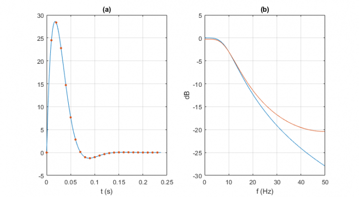
Figure 9.  Discrete-time (red) and continuous-time (blue) responses, impulse-invariant,

ζ = 0.707, f_n= 10 Hz, and f_s = 100 Hz.    a.  Impulse response.    b.  Freq. response magnitude.

Appendix    Matlab Function so_demo.m

The function so_demo.m converts the second-order system H(s) described in Equation 1 to a discrete-time system H(z), and plots the system’s poles, impulse response, and frequency response.  H(z) is shown in Equation 2.  The function call is:

 [K,b,a]= so_demo(zeta,fn,fs,nz);

where

zeta = damping ratio.  zeta > 0 for a stable system.

fn = natural frequency, Hz

fs = sample frequency, Hz

nz = number of zeros (1 or 2)

K = numerator scale factor of H(z)

b = vector of numerator coefficients of H(z)

a = vector of denominator coefficients of H(z)

nz must be 1 or 2:

• For nz = 1, the impulse-invariance method [6] gives a zero at z = 0 + j0.  It turns out that K = T _s*h(T_s), where h(T _s) is the continuous-time system’s impulse response evaluated at t = T_s.  The formula for h(T_s)  varies, depending on whether ζ < 1, ζ = 1, or ζ > 1.  Note that if we didn’t care about exact amplitude scaling, we could have instead set K = sum(a)/sum(b) = sum(a).
• For nz = 2, the zeros are at z = -1 + j0.

Table 1 shows how the function handles the two cases of nz.

For a listing of so_demo.m, see the attached pdf file.

References

1.  Boulet, Benoit, Fundamentals of Signals and Systems, Thomson Learning, 2006, p 300 – 305.

https://mlichouri.files.wordpress.com/2013/10/fundamentals-of-signals-and-systems.pdf

2.  Sachs, Jason, “Second-Order Systems, Part I:Boing!”, Embeddedrelated website, 2014,

https://www.embeddedrelated.com/showarticle/671.php

3.  Signal Processing Toolbox User’s Guide, MathWorks, 2018, p 3.

4.  Signal Processing Toolbox User’s Guide, p 6.

5.  Robertson, Neil, “Design IIR Butterworth Filters Using 12 Lines of Code”, DSPrelated website, 2018,

https://www.dsprelated.com/showarticle/1119.php

6.  Lyons, Richard G., Understanding Digital Signal Processing, 3^rd Ed., section 6.10.

Neil Robertson        April 1, 2020

Sign in