


A Fast Real-Time Trapezoidal Rule Integrator
This blog presents a computationally-efficient network for computing real‑time discrete integration using the Trapezoidal Rule.
Background
While studying what is called "N-sample Romberg integration" I noticed that such an integration process requires the computation of many individual smaller‑sized integrations using the Trapezoidal Rule integration method [1]. My goal was to create a computationally‑fast real‑time Trapezoidal Rule integration network to increase the processing speed of a digital filtering implementation that employs Romberg integration [2].
The Proposed Fast Trapezoidal Rule Integrator
A traditional real‑time N-sample Trapezoidal Rule integrator is shown in Figure 1. That network is real‑time in the sense that when a new x(n) input sample is applied the integrator's y(n) output sample is the N‑sample integration of the current and past (N-1) input x(n) data samples.
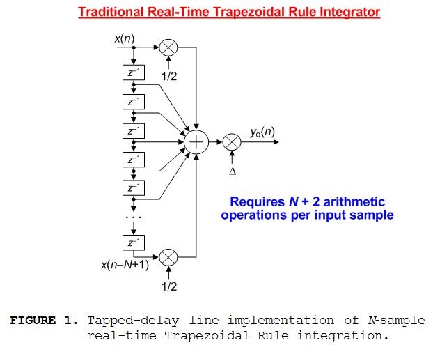
The z-domain transfer function of the Figure 1 network is:
$$H_{o}(z)={Y_{o}(z)\over X(z)}=\Delta\left[{{1\over 2}+z^{-1}+z^{-2}+,...,+z^{-(N-2)}+{z^{-(N-1)}\over 2}}\right].\qquad\qquad\tt(1)$$
For time-domain signals the variable ${\Delta}$ in Figure 1 is:
$${\Delta}={T\over (N-1)}\qquad\qquad\qquad\qquad\qquad\tt(2)$$
where T is the time difference between the x(n) and x(n+N-1) input data samples. A brief review of the Trapezoidal Rule integration method and the derivation of Eq. (1) are given in Appendix A.
The proposed computationally efficient real-time N-sample Trapezoidal Rule integrator, requiring only four arithmetic operations per input sample, is shown in Figure 2.
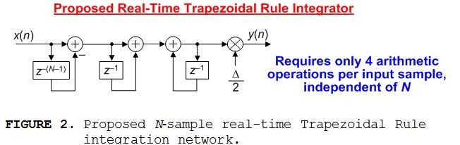
The z‑domain transfer function of that proposed network is:
$$H(z)={Y(z)\over X(z)}={\Delta\over 2}\left[{1+z^{-1}-z^{-(N-1)}-z^{-N}\over 1-z^{-1}}\right].\qquad\qquad\tt(3)$$
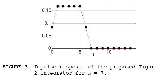
The recursive Figure 2 real-time Trapezoidal Rule integrator has a finite‑length impulse response, shown for N = 7 in Figure 3, and exhibits linear phase because its impulse response is symmetrical (its group delay is a constant (N-1)/2 samples).
Computational Efficiency
The significant computational savings of the proposed Figure 2 integrator, compared to the Figure 1 tapped‑delay line implementation, is illustrated in Figure 4.
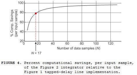
For example, with N = 17 sample trapezoidal integration roughly 79% of the Figure 1 tapped‑delay line implementation's arithmetic operations per input sample are eliminated using the proposed Figure 2 integrator.
Conclusion
We described the computationally‑efficient real‑time Trapezoidal Rule integrator depicted in Figure 2. The integrator's recursive realization is simple, easy to model with signal processing software, and straightforward to implement.
Future Work
What I'd like to do in the future is develop a fast real-time Simpson's Rule integrator.

Acknowledgments
I thank DSP practitioner Paul Lovell for reviewing my original blog manuscript and acknowledge Dr. Balázs Bank of the Budapest University of Technology and Economics. (I developed a real-time integrator requiring five arithmetic operations per input sample. Dr. Bank improved my design resulting in the Figure 2 network requiring only four arithmetic operations per input sample.)
References
[1] Lyons, R., "A Brief Introduction To Romberg Integration", dsprelated.com blog at:
https://www.dsprelated.com/showarticle/1222.php
[2] Henry, M., et. al., "The Prism, Efficient Signal Processing for the Internet of Things", IEEE Industrial Electronics Magazine, December 2017, pp. 22‑32.
Appendix A: A Brief Review of Trapezoidal Rule Integration
The mathematical process of integration has a number of applications in the field of signal monitoring and analysis. As a simple example, we can estimate the instantaneous velocity of a mechanical device by integrating the output signal of an accelerometer attached to that device. Likewise, we can integrate a velocity signal to estimate the instantaneous displacement of a mechanical device. Discrete integration of sampled data is often performed using the Trapezoidal Rule algorithm due to the algorithm's effectiveness and simplicity.
The Trapezoidal Rule is a numerical method used to estimate the area, over the finite‑length time interval b‑a, under an x(t) continuous curve as shown in Figure A‑1. The estimated definite integral is computed using sample values of a finite‑length discrete x(n) sequence (the dots in Figure A‑1).
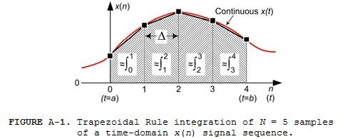
In the Figure A-1 integration example we have a four-segment area, defined by N = 5 x(n) samples, with the sum of those four area segments being our desired approximated integral. (The shaded area between n = 0 and n = 1 in Figure A‑1 is indeed a trapezoid, called a "trapezium" by our friends in the United Kingdom, because it satisfies the condition of being a geometric quadrilateral having at least two parallel sides.)
The area of the first time-domain trapezoid in Figure A-1 is areaa→a+${\Delta}$ ≈ ${\Delta}$[x(0)+x(1)]/2, where
$${\Delta}={b-a\over{N-1}}\tt{seconds.}\qquad\qquad\tt(A-1)$$
Likewise, the area of the second trapezoid in Figure A-1 is: areaa+${\Delta}$→a+2${\Delta}$ ≈ ${\Delta}$[x(1)+x(2)]/2. Including the final two segments, the total area of the four trapezoids in Figure A‑1 (defined by N = 5 x(n) data samples) is:
$$area_{a\to b}\approx\Delta\left[{x(0)+x(1)\over 2}+{x(1)+x(2)\over 2}+{x(2)+x(3)\over 2}+{x(3)+x(4)\over 2}\right]$$
$$\approx\Delta\left[{x(0)\over 2}+x(1)+x(2)+x(3)+{x(4)\over 2}\right]\qquad\qquad\tt(A-2)$$
Based on the Eq. (A-2) example, the general Trapezoidal Rule method for computing discrete integration, based on N x(n) data samples, is expressed as:
$$\int_{a}^{b} x(t)=area_{a\to b}\approx\Delta\left[{x(0)\over 2}+\sum_{k=1}^{N-2} x(k)+{x(N-1)\over 2}\right] \qquad\qquad\tt(A-3)$$
Some people refer to Eq. (A-3) as the "composite Trapezoidal Rule" because it sums the areas of multiple trapezoidal segments.
As you can imagine a larger value of N in Eq. (A‑3), obtained by increasing the sampling rate of x(t) generating more x(n) samples between time instants a and b, will yield a more accurate integral result. The tapped‑delay line implementation of Eq. (A‑3) is that given in this blog's Figure 1.


- Comments
- Write a Comment Select to add a comment

Neat article! I am curious how a trapezoidal integration compares to a boxcar filter (y[k] = average of x[k] through x[k-N]) in terms of signal processing performance.
What I'd like to do in the future is develop a fast real-time Simpson's Rule integrator.
I think I've mentioned this before... Simpson's Rule is great for smooth functions, but it's not really that useful for real digitized data due to the presence of noise and high frequency content.

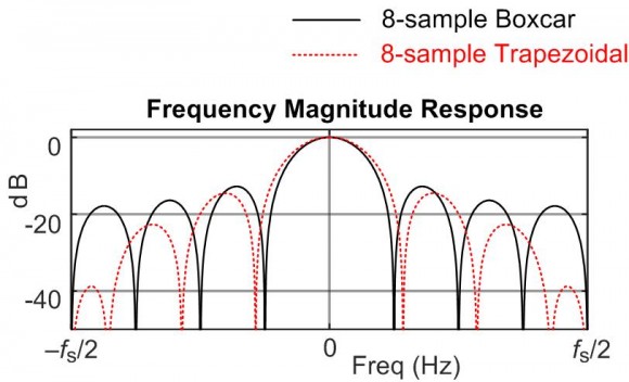
Hi Jason. Both the boxcar filter and my Figure 2 Trapezoidal integrator are lowpass filters. But the Trapezoidal integrator's impulse response is equivalent to a "windowed" boxcar filter's impulse response. So the Trapezoidal integrator's frequency response will, as expected, have a wider mainlobe and lower sidelobes compared the frequency response of a boxcar filter as shown below.
Hi Rick,
In equation 1, you have "H(z) = \delta (1/2 + X(z) z^-1 + ..."; unless I've missed something, the X(z) is a mistake (maybe it got left in while the function was being changed from Y(z) = to H(z) = in editing?).
Hi ziph. You are correct! That factor X(z) in Eq. (1) is a typographical error caused by my lack of skills in using MathJax syntax. Thankfully the error is absent in this blog's associated PDF file. ziph, I've corrected the error in my blog and thanks for pointing out that error to me!
To post reply to a comment, click on the 'reply' button attached to each comment. To post a new comment (not a reply to a comment) check out the 'Write a Comment' tab at the top of the comments.
Please login (on the right) if you already have an account on this platform.
Otherwise, please use this form to register (free) an join one of the largest online community for Electrical/Embedded/DSP/FPGA/ML engineers:


