A Brief Introduction To Romberg Integration

This blog briefly describes a remarkable integration algorithm, called "Romberg integration." The algorithm is used in the field of numerical analysis but it's not so well-known in the world of DSP.

To show the power of Romberg integration, and to convince you to continue reading, consider the notion of estimating the area under the continuous x(t) = sin(t) curve based on the five x(n) samples represented by the dots in Figure 1.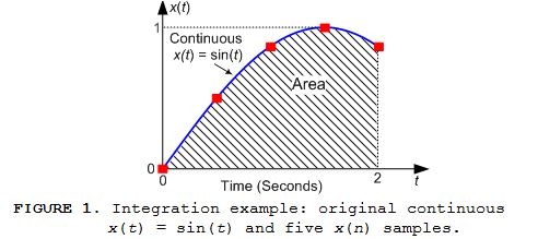

The results of performing a Trapezoidal Rule, a Simpson's 1/3 Rule, and a Romberg integration using Figure 1's five x(n) samples are given in Table 1. There we see the profound reduction in integration error afforded by Romberg integration.

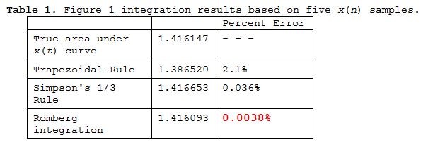
To achieve Table 1's low 0.0038% Romberg error a Trapezoidal Rule integration would require 100 x(n) samples rather than just the five x(n) samples in Figure 1. To learn more about Romberg integration please read on.

Romberg Integration

Romberg integration is a process used to compute finite integrals requiring very high accuracy (super‑low error). This integration process, first proposed by Werner Romberg in 1955, is remarkable because it employs a series smaller‑sized less‑accurate integral approximations, typically obtained using the Trapezoidal Rule integration method, to compute a much more accurate final definite integral approximation [1-3].

A simplified depiction of the Romberg integration process used to compute the Romberg integration values in the bottom row of Table 1 is shown in Figure 2.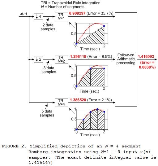

The 'TRI' notation in Figure 2 means Trapezoidal Rule integration and the ↓k symbol represents downsampling by integer k. We see in Figure 2 that separate four-segment, three-segment, and two-segment Trapezoidal Rule integrations are performed.

Figure 2 is called an "N = 4-segment Romberg integration" because five input x(n) samples enables the total integrated area to be divided into N = 4 smaller area segments as shown by the bottom integration in Figure 2. As it turns out, log₂(N)+1 individual trapezoidal integration operations are required for a single N-segment Romberg integration process.

The full block diagram of the N = 4-segment Romberg integration is given in Figure 3.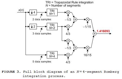

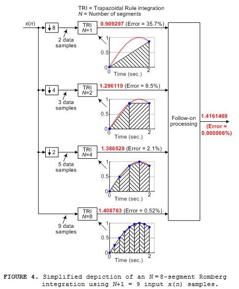
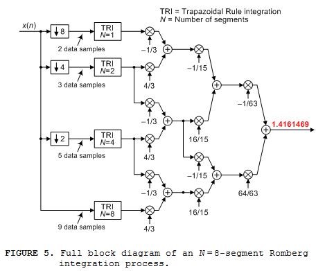
If we had nine x(n) signal samples of Figure 1's continuous x(t) signal, between t = 0 and t = 2 seconds, we could perform the N = 8‑segment Romberg integration shown in Figure 4. In that case our computed integral value is 1.4161469 having a percent error of 6x10^‑6%.

The full block diagram of the N = 8-segment Romberg integration is given in Figure 5.

An N = 16 Integration Example

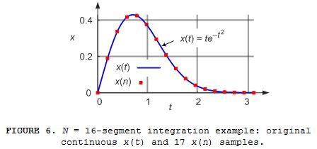
Below I present the N = 16‑segment (17 signal samples) estimated definite integral of the continuous x(t), over the time range of 0 ≤ t ≤ p, defined by:

shown in Figure 6.

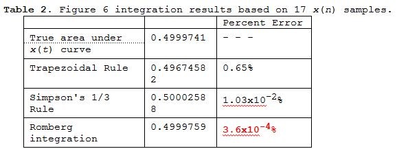
The Figure 6 estimated integral results are given in Table 2. There we see the improved accuracy, for this particular x(n) sequence, of our Romberg integration. To achieve Table 2's 3.6x10^-4% Romberg error a Trapezoidal Rule integration would require 680 x(n) samples rather than just the 16 x(n) samples in Figure 6.

To keep this blog from being too lengthy I conclude my discussion here. If Romberg integration interests you, the following additional information 

Further details, and references, regarding Romberg integration

How to compute the multiplication coefficients in Figures 3 and 5

Additional Romberg integration examples

 MATLAB code implementing Romberg integration

is available in this → downloadable PDF file:

                  

Sign in