Add a Power Marker to a Power Spectral Density (PSD) Plot

• Matlab
• DFT_FFT

Perhaps we should call most Power Spectral Density (PSD) calculations relative PSD, because usually we don’t have to worry about absolute power levels.  However, for cases (e.g., measurements or simulations) where we are concerned with absolute power, it would be nice to be able to display it on a PSD plot.  Unfortunately, you can’t read the power directly from the plot.  For example, the plotted spectral peak of a narrowband signal, such as a sinewave, is lower than the actual power, due to the processing loss of the DFT’s window function [1-3].  And for a modulated signal, e.g., QAM or OFDM, the spectrum occupies many DFT bins, and the total power is not obvious.

In this post, I provide a Matlab function psd_mkr that computes the PSD, plots the spectrum, and displays power using a marker.  There are three marker modes:

• Normal mode, for narrowband signals like sinewaves.
• Band-power mode, which displays the power over a specified band (useful for modulated signals).
• 1 Hz mode, for displaying power in a 1 Hz bandwidth.

See Appendix A of the PDF version for the Matlab code.  The function uses the Matlab function pwelch [4] to compute the PSD.  I discussed pwelch in an earlier post [5].

Function Call

The function call to psd_mkr is as follows:

    [PdB_mkr,PdB,f]= psd_mkr(x,nfft,fs,ref_dBW,f_mkr,bw_mkr);
    where
        x = discrete-time signal vector, Volts (real).
        nfft = number of frequency samples, 0 to fs.
        fs = sample rate, Hz.
        ref_dBW = reference level for plot, dB-Watts.
        f_mkr = marker frequency, Hz.
        bw_mkr = bandwidth over which power is measured, Hz.  
                 Setting bw_mkr = 0 (or omitting it) invokes normal mode.
 .
        PdB_mkr = power over marker bandwidth, dBW (1 ohm).
        PdB = PSD vector, dBW.  Length = nfft/2 + 1.
        f = frequency vector, Hz.  Range = 0 to fs/2.

The spectrum plot’s vertical range is 100 dB.  Given a signal x of length N, setting nfft = N results in a PSD without DFT averaging.  If N is a multiple of nfft, DFT averaging is performed [4, 5].  The power in dBW is calculated assuming a resistance of 1 ohm.

Note that you can plot two markers by calling psd_mkr twice, specifying a different marker frequency each time.  You must issue the command "hold on" after the first call to psd_mkr.  As an example, you can use two band-power markers to compute a modulated signal’s adjacent channel power ratio (ACPR).

Appendix B of the PDF version lists the Matlab function psd_mkr_dBm, which is identical to psd_mkr, except the power is computed in dBm (dB-milliwatts), and the load resistance is 50 ohms.

Example 1 – Normal Mode

Here is an example that uses psd_mkr in normal mode.The signal is a sinewave plus Gaussian noise.Sine amplitude A is sqrt(2), with power into 1 ohm of A²/2 = 1 Watt = 0 dBW.  The Matlab code to generate the signal and plot the spectrum with marker is as follows:

    fs= 2000;                       % Hz sample frequency
    Ts= 1/fs;
    f0= 300;                        % Hz sine frequency
    A= sqrt(2);                     % sine amplitude (P= 1 Watt)
    N= 8192;                        % number of time samples
    n= 0:N-1;                       % time index
    x= A*sin(2*pi*f0*n*Ts) + .01*randn(1,N);    % signal with noise
    nfft= 2048;                     % number of frequency samples, 0 to fs
    ref_dBW= 10;                    % dBW reference level for plot
    f_mkr= f0;                      % Hz marker frequency
    psd_mkr(x,nfft,fs,ref_dBW,f_mkr);

The plot generated by psd_mkr is shown in Figure 1.  As expected, the marker value is 0 dBW.  Note that the peak of the spectrum is only about -2.5 dBW, due to the processing loss of the function’s Kaiser window.

The function calculates the marker level by adding the power of several bins closest to f₀ = 300 Hz.  This is shown in Figure 2, where we have zoomed in on the spectral peak, and plotted the spectrum magnitude (before conversion to dBW) using a linear amplitude scale.  The spectrum is the convolution of the window’s spectrum and the sine spectrum, which causes the power to be spread over several bins.  In psd_mkr, we sum the contributions of the five bins shown in red to compute the marker value of 1 Watt = 0 dBW.  In the code listing of Appendix A (see PDF version), this is performed by the line:

    p_mkr= fs/nfft*sum(pxx(k1:k2));       % W (Hz/bin* W/Hz* bins)

Keep in mind that normal mode is only appropriate for narrowband signals with bandwidth (prior to windowing) of less than one bin.  For a signal that occupies several bins, use band-power mode instead.

As mentioned, psd_mkr uses the Matlab function pwelch to calculate the PSD.  Note that pwelch calculates the PSD in W/Hz.  psd_mkr converts these units to W/bin using the following formulas:

Pbin (W/bin) = pxx (W/Hz) * fs/nfft (Hz/bin)

PdB (dBW/bin) = 10*log10(Pbin)

If you are interested in the math involved to find the power of DFT spectral components, see my post: “The Power Spectrum” [6].

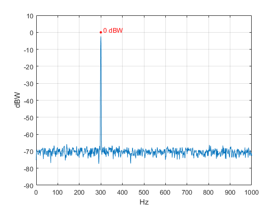
Figure 1.  Demonstration of normal marker mode.

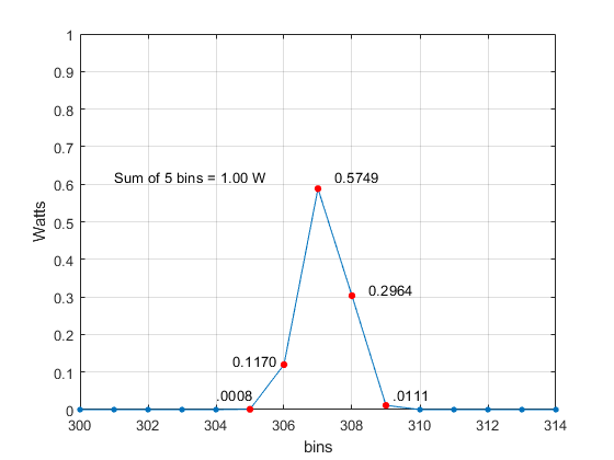
Figure 2.  Close-in Spectrum of 1-Watt sinusoid of Example 1, showing power of individual

DFT bins, linear amplitude scale.  Window function = Kaiser(N,8).

Example 2 -- Band Power Mode

In Band Power mode, the function call is the same as above, except we include the parameter bw_mkr, which is the bandwidth in Hz over which the power is measured.  f_mkr is the center of the band.  To measure the power, the function simply adds the power in the bins corresponding to the specified center frequency and bandwidth.

This example finds the power over a band that includes two sinewaves at 300 and 400 Hz, each with level of 0 dBW.  To display the total power, we set f_mkr = 350 Hz and bw_mkr= 125 Hz.  The Matlab code is as follows:

    fs= 2000;                  % Hz sample frequency
    Ts= 1/fs;
    f0= 300;                   % Hz sine #1 frequency
    f1= 400;                   % Hz sine #2 frequency
    A= sqrt(2);                % sine amplitude (P= 1 Watt)
    N= 8192;                   % number of time samples
    n= 0:N-1;                  % time index
    x= A*sin(2*pi*f0*n*Ts) + A*sin(2*pi*f1*n*Ts)+ .01*randn(1,N);
    nfft= 2048;                % number of frequency samples, 0 to fs
    ref_dBW= 10;               % dBW reference level for plot
    f_mkr= 350;                % Hz marker frequency
    bw_mkr= 125;               % Hz marker bandwidth
    psd_mkr(x,nfft,fs,ref_dBW,f_mkr,bw_mkr);

The plot generated by psd_mkr is shown in Figure 3.  Each sinusoid has power of 1 watt, so the band power is 10*log₁₀(2 W) = 3.01 dBW.  As shown, the band-power marker is a horizontal red line, centered at f_mkr, with length bw_mkr.  To view more detail, we can specify the axes as follows:

    axis([250 450 -10 10])

This gives the plot shown in Figure 4.  Note that the peak levels of the two PSD frequency components differ by about 0.5 dB; this is due to DFT scalloping [1].  Scalloping has no effect on the band power calculation.

The band power mode is particularly useful for modulated signals.  Figure 5 demonstrates band power mode for a QAM signal.

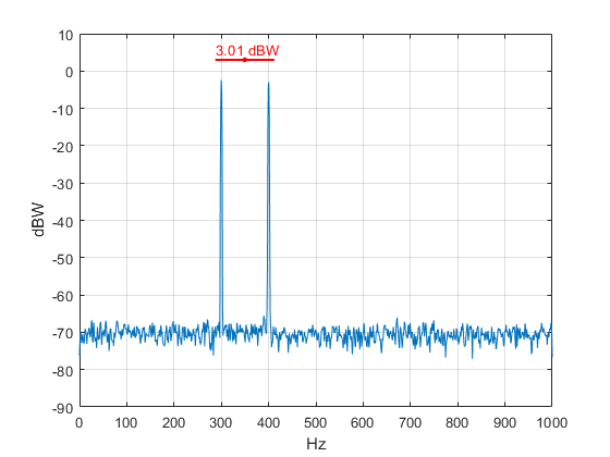
Figure 3.  Power of two 0 dBW sinewaves using band power mode.

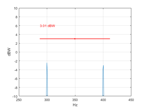
Figure 4.  Detail view of Figure 3, using  axis([250 450 -10 10])

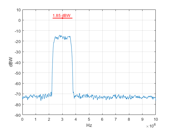
Figure 5.  Power of a QAM signal using band power mode.

Example 3 -- 1 Hz Mode

To use 1 Hz mode, set bw_mkr = 1.  The spectrum is then plotted twice, in units of dBW and dBW (1 Hz), with marker units of dBW (1 Hz).  In this example, we use the 1 Hz mode to measure noise power density.  The signal is a sinewave plus Gaussian noise.  The Matlab code is as follows:

    fs= 1e6;                     % Hz sample frequency
    Ts= 1/fs;
    f0= 200E3;                    % Hz sine frequency
    A= sqrt(2);                   % sine amplitude (P= 1 Watt)
    N= 8192;                      % number of time samples
    n= 0:N-1;                     % time index
    x= A*sin(2*pi*f0*n*Ts) + .02*randn(1,N);    % signal with noise
    nfft= 512;                    % number of frequency samples
    ref_dBW= 0;                   % dBW reference level for plot
    f_mkr= 300E3;                 % Hz marker frequency
    bw_mkr= 1;                    % Hz
    psd_mkr(x,nfft,fs,ref_dBW,f_mkr,bw_mkr);

The Matlab function generates the PSD shown in Figure 6, where the blue spectrum is in dBW/bin and the grey spectrum is in dBW/Hz.  The number of time-samples is 8192, while nfft is 512.  This causes DFT averaging of several FFT’s, reducing the variance of the noise.  The marker shows the noise level at 200 kHz as – 91.7 dBW (1 Hz).  The signal level is 0 dBW, so C/N₀ = 0 - -91.7= 91.7dB (1 Hz).

Incidentally, the amplitude offset between the two plots in Figure 6 depends on the ratio of the power in W/Hz to that in W/bin:

$$ R= \frac{W/Hz}{W/bin}  = \frac{bins}{Hz} = \frac{nfft}{f_s} $$

In dB:

$$ R_{dB}= 10*log_{10}(nfft/f_s) $$

For our example, nfft = 512 and f_s = 1E6.  Thus R_dB = -32.9 dB, and the spectrum in dBW (1 Hz) is 32.9 dB lower than the one in dBW.

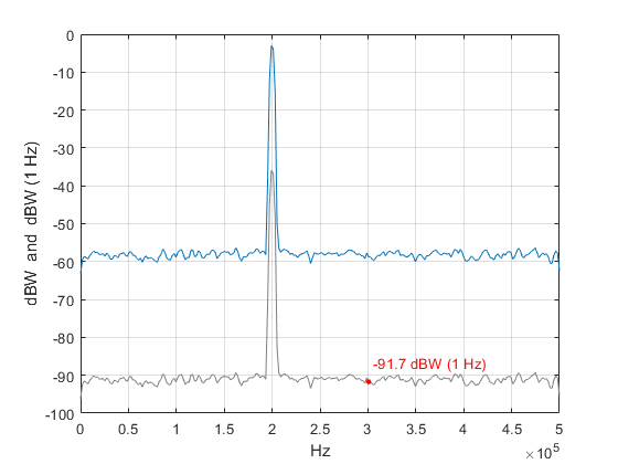
Figure 6.  Using 1 Hz mode to measure noise power density.

Blue = dBW, grey = dBW (1Hz).

For Appendices, see the PDF version of this article.

References

1.  Robertson, Neil, “Evaluate Window Functions for the Discrete Fourier Transform”, DSPrelated.com, Dec, 2018, https://www.dsprelated.com/showarticle/1211.php

2.  Rapuano, Sergio, and Harris, Fred J., An Introduction to FFT and Time Domain Windows, IEEE Instrumentation and Measurement Magazine, December, 2007,              https://ieeexplore.ieee.org/document/4428580

3.  Harris, Fredric J., “On the Use of Windows for Harmonic Analysis with the Discrete Fourier Transform”, Proc. IEEE, vol 66, pp. 51-83, Jan 1978.    https://www.utdallas.edu/~cpb021000/EE%204361/Great%20DSP%20Papers/Harris%20on%20Windows.pdf

4.  The Mathworks website, https://www.mathworks.com/help/signal/ref/pwelch.html

5.  Robertson, Neil, “Use Matlab Function Pwelch to Find Power Spectral Density – or Do It Yourself”, DSPrelated.com, Jan, 2019, https://www.dsprelated.com/showarticle/1221.php

6.  Robertson, Neil, “The Power Spectrum”, DSPrelated.com, Oct, 2016, https://www.dsprelated.com/showarticle/1004.php ,

7. The Mathworks website,https://www.mathworks.com/help/signal/ug/kaiser-window.html

Neil Robertson      February, 2021

Sign in