


A Differentiator With a Difference
Some time ago I was studying various digital differentiating networks, i.e., networks that approximate the process of taking the derivative of a discrete time-domain sequence. By "studying" I mean that I was experimenting with various differentiating filter coefficients, and I discovered a computationally-efficient digital differentiator. A differentiator that, for low fequency signals, has the power of George Foreman's right hand! Before I describe this differentiator, let's review a few fundamentals of simple digital differentiators.
Digital Differentiation
While the idea of differentiation is well-defined in the world of continuous signals, the notion of differentiation is not well defined for discrete signals. However, fortunately we can approximate the calculus of a derivative operation in the domain of discrete signals. (While DSP purists prefer to use the terminology digital differencer, here I'll use the phrase differentiator.) To briefly review the notion of differentiation, think about a continuous sinewave, whose frequency is ω radians/second, represented by
| | (1) |
The derivative of that sinewave is
| (2) |
So the derivative of a sinewave is a cosine wave whose amplitude is proportional to the original x(t) sinewave's frequency. Equation (2) tells us that an ideal differentiator's frequency magnitude response is a straight line increasing with frequency ω. With that thought in mind, I'll now mention two common discrete-time FIR (nonrecursive) differentiators: a first-difference and a central-difference differentiator. They are computationally simple schemes for estimating the derivative of a digital x(n) time-domain signal sequence with respect to time.
The first-difference differentiator, the simple process of computing the difference between successive x(n) signal samples, is defined in the time domain by
| (3) |
The frequency magnitude response of that differentiator is the dashed |Hfd(ω)| curve in Figure 1(a). (For comparison reasons, I also show an ideal differentiator's straight-line |Hideal(ω)| = ωmagnitude response in Figure 1(a). The frequency axis in that figure covers the positive frequency range 0 ≤ω≤ π samples/radian, corresponding to a cyclic frequency range of 0 to fs/2, where fs is the x(n) sample rate in Hz.) Equation (3) is sweet in its simplicity but unfortunately its |Hfd(ω)| tends to amplify high-frequency noise that often contaminates real-world signals. For that reason the central-difference differentiator is often used in practice.
The time-domain expression of the central-difference differentiator is
| | (4) |
The central-difference differentiator's frequency magnitude response is the dotted |Hcd(ω)| curve in Figure 1(a). The price we pay for |Hcd(ω)|'s desirable high-frequency (noise) attenuation is that its frequency range of linear operation is only from zero to roughly ω = 0.16π samples/radian (0.08fs Hz) which is, unfortunately, less than the frequency range of linear operation of the first-difference differentiator.
Here's the Beef
Now, ... for the computationally-efficient differentiator that maintains the central-difference differentiator's beneficial high-frequency attenuation behavior, but extends its frequency range of linear operation. The differentiator that I'm promoting is defined by
| (5) |
This novel differentiator's normalized magnitude response is the solid |Hdif(ω)| curve in Figure 1(a), where we see that its frequency range of linear operation extends from zero to approximately ω= 0.34π samples/radian (0.17fs Hz). The ydif(n) differentiator is twice the usable frequency range of the central-difference differentiator.
The implementation of the ydif(n) differentiator is shown in Figure 1(b) where a delay block comprises two unit delays. The folded-FIR block diagram for this differentiator is presented in Figure 1(c) where only a single multiply need be performed per ydif(n) output sample. The really slick aspect of the ydif(n) differentiator is that its non-unity coefficients (±1/16) are integer powers of two. This means that a multiplication in Figure 1 can be implemented with an arithmetic right shift by four bits. Happily, such a binary right-shift implementation is a linear-phase multiplierless differentiator!

Figure 1: Efficient differentiator: (a) performance; (b) standard block diagram; (c) folded block diagram.
Another valuable feature of the Equation (5) ydif(n) differentiator is that its time delay (group delay) is exactly three sample periods (3/fs). Having a delay that's an integer number of samples makes this differentiator convenient when the differentiator's output must be synchronized with other time-domain sequences, such as for use with popular FM demodulation methods.
[Sept. 2015 Note: I've written a more recent blog regarding another interesting differentiator. That blog is at:
http://www.dsprelated.com/showarticle/814.php ]
Copyright © 2007, Richard Lyons, All Rights Reserved


- Comments
- Write a Comment Select to add a comment

I have no mathematical derivation for the simple digital differentiator described in this blog. Years ago I was looking at DSP pioneer Richard Hammings 1998 book titled: Digital Filters. I looked at his simple differentiators, one of which had the coefficients: -1/6,8/6,0,-8/6, and 1/6. I thought, Gee. It would be nice if the denominator was an 8 instead of a 6 -- then the division be could be replaced by a binary right shift of three bits. After that, like Thomas Edison trying to find the right material for his light bulbs filament, I merely started experimenting with various simple differentiator coefficients (having alternating +/- signs) whose denominators were an integer power of two. I finally stumbled upon the coefficients described in this blog. Joseph, beware. If I recall correctly, the differentiator described in this blog has a linear gain of 1.68 rather than an ideal differentiators gain of one.
[-Rick-]
I did not see your comment until today. Sorry for being 10 months late! Try the following code:
A=1;
B = [-1/16, 0, 1, 0 -1, 0 1/16];
[H,W] = freqz(B,A,256,'whole');
H_mag = abs(H)';
Freq = (-length(H)/2:length(H)/2-1)/length(H);
plot(Freq,H_mag,'k'), grid on
ylabel('Linear'), title('Mag. Response'), zoom on
xlabel('Freq. (times Fs)')
[-Rick-]

Hi Rick,
I modified your code to compute the response over 0 to pi. If I then plot the magnitude, the slope is not 1, see plot below. Am I doing something wrong?
thanks,
Neil
A=1;
B = [-1/16, 0, 1, 0 -1, 0 1/16];
[H,W] = freqz(B,A,256);
H_mag = abs(H)';
plot(W,H_mag,W,W),grid
axis([0 pi 0 pi])
xlabel('\omega')
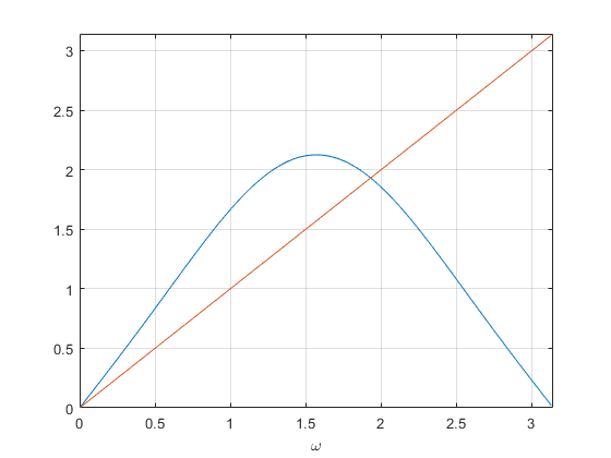
Hi Neil. You are correct.
I failed to say that my Figure 1 differentiator’s gain is greater than one. The black curve in my Figure 1(a) is normalized by the “Ideal” differentiator’s magnitude response. That is, I multiplied my differentiator’s magnitude response by 0.6 to plot the black curve in Figure 1(a). Sorry for the confusion Neil.
OK, I thought that might be the case.
regards,
Neil
So, it's 9 years later and I have a question...
I have your book and I just got to chapter 7, which includes a discussion of differentiators. I couldn't figure out a couple paragraphs and I googled, which led me here.
You say the FD method "amplifes" the high frequencies, but the CD "attenuates". I don't understand this at all. Both the FD and CD curves are everywhere below the IDEAL straight line.
Also, unlike in much of the rest of the book, there's no explanation of what practical use the derivative of a signal is. What does that even mean? I guess it's the rate at which different frequency bands are appearing or disappearing from the total signal? Like "attack" and "decay"?
(I wrote this blog nine years ago(!)? Good Lord, where did those nine years go?)
To expand on my words "amplify" and "attenuate", have a look at the above Figure 1. At high frequencies, the $|H_{fd}{(\omega)}|$ curve has a higher gain than does the $|H_{cd}{(\omega)}|$ curve. When we want to compute the instantaneous derivative of a low-frequency signal-of-interest we usually do NOT want to amplify any high-frequency background noise that's contaminating that signal. So a digital differentiator that has a linear gain (linear versus frequency) at low frequencies and low gain at high frequencies is desirable.
By the way, I have another differentiator blog at:
https://www.dsprelated.com/showarticle/814.ph
As for practical applications of digital differentiators, differentiation is a key step in one the traditional methods of FM demodulation. Think of an application where you're measuring the rotational velocity of a metal shaft and producing a velocity signal $v(n)$. If you need to know the instantaneous rotational acceleration of the shaft then you'd differentiate merely differentiate your $v(n)$ signal. I imagine image processing guys use differentiation in some of their applications.
drysdam, if you have a hardcopy of my DSP book you can send me a private e-mail, at R_dot_Lyons_at_ieee_dot_org, and we can arrange for me to send you the errata for your copy of my book. It's up to you.
Hi Rick,
Is there similar technique available for complex signals? I am currently looking into Teager Energy operators, which requires first and second order differentiation on complex signals. But first-difference operation (x[n] – x[n-1]) is very sensitive to noise. I believe a higher order approximation (either FIR or non-linear approach) is the way to go. But I am not sure if they are applicable to complex signals.
Hi wildchild.
To differentiate a complex signal 'x(n)' we merely differentiate the real and imaginary parts of 'x(n)' separately as shown by the following diagram:
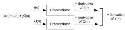
The "Differentiators" in the above diagram must be identical networks and they can be, for example, this blog's noise-limiting Figure 1 differentiator or possibly the noise-limiting differentiator in Figure 3 at:
https://www.dsprelated.com/showarticle/814.php
There are higher-order noise-limiting FIR differentiators available with improved performance. But, of course, they require more computations per output sample.
"Teager Energy
operators" huh? I don't recall ever hearing about that particular signal processing subject. Maybe I'll try to learn something about them in the future.
To post reply to a comment, click on the 'reply' button attached to each comment. To post a new comment (not a reply to a comment) check out the 'Write a Comment' tab at the top of the comments.
Please login (on the right) if you already have an account on this platform.
Otherwise, please use this form to register (free) an join one of the largest online community for Electrical/Embedded/DSP/FPGA/ML engineers:


