A New Contender in the Digital Differentiator Race

This blog proposes a novel differentiator worth your consideration. Although simple, the differentiator provides a fairly wide 'frequency range of linear operation' and can be implemented, if need be, without performing numerical multiplications.

---

---

Background

In reference [1] I presented a computationally-efficient tapped-delay line digital differentiator whose $h_{ref}(k)$ impulse response is:

$$ h_{ref}(k) = {-1/16}, \ 0, \ 1, \ 0, \ {-1}, \ 0, \ 1/16 \tag{1} $$

and whose $ \lvert H_{ref}(\omega) \rvert $ frequency magnitude response is shown by the blue dashed curve in Figure 1.

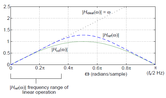
Figure 1: Normalized frequency magnitude responses of
the reference [1] differentiator, and a
central-difference differentiator.

For comparison purposes, Figure 1 shows the frequency magnitude response of the popular central-difference differentiator (green dotted curve), $ \lvert H_{cd}(\omega) \rvert $, whose $h_{cd}(k)$ impulse response is:

$$ h_{cd}(k) = 1/2, \ 0, \ {-1/2}. \tag{2} $$

In Figure 1 we see the $ \lvert H_{ref}(\omega) \rvert $ response's increased 'frequency range of linear operation' compared to the $ \lvert H_{cd}(\omega) \rvert $ frequency magnitude response. That's the primary benefit of the $h_{ref}(k)$ differentiator.

The response curves in Figure 1 are what I call "normalized" magnitude responses. I'll define what I mean by normalized later in this blog.

(As a bit of trivia, it's interesting to note that the central-difference differentiator's magnitude response is equal to the first half cycle of a sine wave. I prove that fact in Appendix A.)

The Proposed Differentiator

The improved differentiator I propose here has the impulse response given by:

$$ h_{pro}(k) = {-3/16}, \ 31/32, 0, \ {-31/32}, \ 3/16 \tag{3} $$

and whose $ \lvert H_{pro}(\omega) \rvert $ frequency magnitude response is shown by the black solid curve in Figure 2.

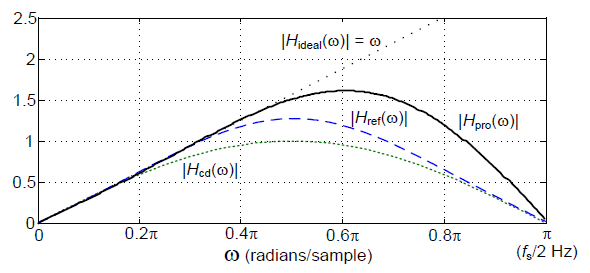
Figure 2: Normalized frequency magnitude responses of
the proposed differentiator, the reference [1]
differentiator, and a central-difference
differentiator.

Figure 2 shows the benefit of the proposed $ h_{pro}(k) $ differentiator. Its $ \lvert H_{pro}(\omega) \rvert $ response has an increased-width (by roughly 33%) 'frequency range of linear operation' compared to the $ \lvert H_{ref}(\omega) \rvert $ frequency magnitude response. Based on Figure 2, the $ h_{pro}(k) $ differentiator should be useful in applications where the spectral components of the input signal are less than $ \pi/2 $ radians/sample $ (f_s/4 \ Hz.) $

The $ h_{pro}(k) $ differentiator has, due to its antisymmetrical coefficients, linear phase in the frequency domain. In addition, the differentiator's input/output time delay (group delay) is exactly two sample periods. Having a delay that's an integer number of samples makes this differentiator useful when its output must be synchronized with other time-domain sequences, such as in FM demodulation applications.

Proposed Differentiator Implementation

The traditional tapped-delay line implementation of the proposed differentiator is shown in Figure 3(a). A folded delay line implementation reducing the number of computations from four multiplications to two multiplications per output sample is given in Figure 3(b). And a folded multiplier-free implementation is shown in Figure 3(b) where multipliers are replaced by binary right-shift operations. In that figure the 'BRS,x' nomenclature means a binary right shift by x bits.

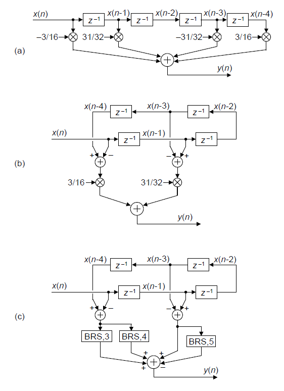
Figure 3: Proposed $ h_{pro}(k) $ differentiator implementations:
(a) traditional implementation; (b) folded
implementation; (c) folded multiplier-free
implementation.

Differentiator Gains and Normalized Magnitude Curves

For completeness I mention that the $ h_{ref}(k) $ and $ h_{pro}(k) $ differentiators have magnitude response gains greater than unity. This is shown by the actual frequency magnitude responses shown in Figure 4.

To explain what I mean by "gain", notice how the slope of the central-difference differentiator's $ \lvert H_{cd}(\omega) \rvert $ response (green dotted) curve is unity at low frequencies in Figure 4. Thus I claim the gain of the $ h_{cd}(k) $ differentiator has a gain of one. The slope of the reference [1] differentiator's $ \lvert H_{ref}(\omega) \rvert $ response (blue dashed) curve is 1.63 at low frequencies and the slope of the proposed differentiator's $ \lvert H_{pro}(\omega) \rvert $ response (black solid) curve is 1.2 at low frequencies. So I claim that the $h_{ref}(k)$ reference [1] and $ h_{pro}(k) $ proposed differentiators have gains of 1.63 and 1.2 respectively.

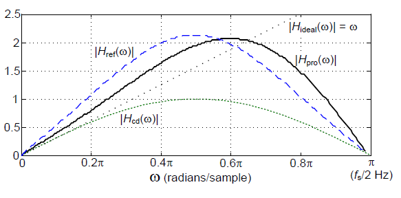
Figure 4: Actual frequency magnitude responses of
the proposed differentiator, the reference [1]
differentiator, and a central-difference
differentiator.

Those actual magnitude response curve in Figure 4 prevent us from comparing the 'frequency ranges of linear operation' of the various differentiators. So to make that comparison I divided the Figure 4 $ \lvert H_{ref}(\omega) \rvert $ response sample values by 1.63 to create the normalized blue dashed curves in Figures 1 and 2. Likewise, I divided the Figure 4 $ \lvert H_{pro}(\omega) \rvert $ response sample values by 1.2 to create the normalized solid black curve in Figure 2.

A Digital Differentiator Clarification

When thinking about digital differentiators it's useful to be aware of the algebraic form of their time-domain difference equations. For example, let's assume that $ y(n) $ represents a central-difference derivative of an $ x(n) $ sequence. The correct estimation of the $ y(n) $ derivative of an $ x(n) $ is:

$$ \text{estimated derivative of } x(n) = y(n) = {{x(n) - x(n-2)} \over {2t_s}} \tag{4} $$

where $ t_s $ is the time between the $ x(n) $ samples measured in seconds. (Variable $ t_s $ is the 'dt' in a generic differentiator's dx/dt derivative.)

Often in the DSP literature, for convenience, the time between $ x(n) $ samples is assumed to be unity, i.e. $ t_s = 1 $ and a central-difference differentiator's difference equation takes the popular form of:

$$ y'(n) = {{x(n) - x(n-2)} \over 2} . \tag {5} $$

Computing Eq. (5)'s estimated $ y'(n) $ derivative is acceptable in many applications because $ y'(n) $ will always be proportional to Eq. (4)'s $ y(n) $. But to be dimensionally correct, Eq. (4)'s $ y(n) $ should be computed, rather than Eq. (5)'s $ y'(n) $.

For example, let's say the continuous red-dotted curve in Figure 5 is the $ x(t) $ instantaneous water pressure inside a water pipe measured in pounds per square inch (psi). And we have three $ x(n) $ samples of $ x(t) $ shown by the large $ x(n) $ black dots. The $ t_s $ time between sample is 0.5 seconds.

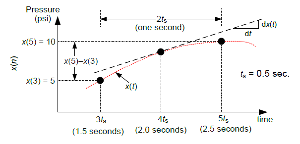
Figure 5: Digital differentiator example. Estimating the
slope, $ dx(t)/dt $, of the continuous $ x(t) $ signal
by way of digital differentiation of the
sampled $ x(n) $ sequence.

To estimate the rate of pressure change at time instant two seconds $ (4t_s) $ once sample $ x(5) $ is available, using Eq. (5) gives us a $ y'(5) $ value of:

$$ y'(5) = {{x(5)-x(3)} \over 2} = {{10 \ psi - 5 \ psi} \over 2} = 2.5 psi. $$

However, time rate of pressure change values must dimensionally be psi/second.

What we should do is use Eq. (4) giving us a dimensionally-correct time rate of pressure change value of:

$$ y(5) = {{x(5) - x(3)} \over {2t_s \ seconds}} = {{10 \ psi - 5 \ psi} \over {1 \ second}} = 5 \ psi/second. $$

Result $ y(5) $ tells us the water pressure increased by 5 psi during the one-second time interval from 1.5 seconds to 2.5 seconds. So my point is, Eq. (5)'s $ y'(n) $ is the popular form of a central-difference differentiator's difference equation, but Eq. (4)'s $ y(n) $ expression is the dimensionally-correct form.

References

[1] http://www.dsprelated.com/showarticle/35.php

Appendix A: Proof of Cent-Diff Differentiator's Sinusoidal Magnitude Response

The proof that a central-difference differentiator's magnitude response is equal to the magnitude of a sine wave proceeds as follows: With the differentiator's time-domain impulse response being $ h_{cd}(k) = [1/2, \ 0, \ -1/2] $, its z-transform is

$$ H_{cd}(z) = {{z^{-0} - z^{-2}} \over 2} . \tag{A-1} $$

Multiplying Eq. (A-1) by $ z/z $ gives us a new, and equivalent, z-transform of:

$$ H_{cd}(z) = {1 \over z}{{z^{1} - z^{-1}} \over 2} . \tag{A-2} $$

Replacing $ z $ with $ e^{j\omega} $ gives us the differentiator's frequency response of:

$$ H_{cd}(\omega) = {1 \over {e^{j\omega}}}{{e^{j\omega} - e^{-j\omega}} \over 2} . \tag{A-3} $$

Knowing that $ (e^{-j\omega} -e^{-j\omega})/2 = jsin(\omega) $, we write:

$$ H_{cd}(\omega) = {j \over {e^{j\omega}}}[sin(\omega)] = {{e^{j\pi/2}} \over {e^{j\omega}}}[sin(\omega)] . \tag{A-4} $$

Therefore the $ \lvert H_{cd}(\omega) \rvert $ frequency magnitude response is equal to the magnitude of a sine wave as:

$$ \lvert H_{cd}(\omega) \rvert = \left\lvert\frac{e^{j\pi/2}}{e^{j\omega}}[sin(\omega)]\right\rvert = \left\lvert {e^{-j(\omega-\pi/2)}[sin(\omega)]} \right\rvert = \lvert sin(\omega) \rvert . \tag{A-5} $$

---

Previous post by Rick Lyons:
   The Most Interesting FIR Filter Equation in the World: Why FIR Filters Can Be Linear Phase
Next post by Rick Lyons:
   Implementing Simultaneous Digital Differentiation, Hilbert Transformation, and Half-Band Filtering

Sign in