It is possible to compute N-point discrete Fourier transforms (DFTs) using radix-2 fast Fourier transforms (FFTs) whose sizes are less than N. For example, let's say the largest size FFT software routine you have available is a 1024-point FFT. With the following trick you can combine the results of multiple 1024-point FFTs to compute DFTs whose sizes are greater than 1024.

The simplest form of this idea is computing an N-point DFT using two N/2-point FFT operations. Here's how the trick works for computing a 16-point DFT, of a 16-sample x(n) input sequence, using two 8-point FFTs; we execute the following steps:

1. Perform an 8-point FFT on the x(n) samples where n = 0, 2, 4, ..., 14. We'll call those FFT results X₀(k).
2. Store two copies of X₀(k) in Memory Array 1 as shown in Figure 1.
3. Next we compute an 8-point FFT on the x(n) samples where n = 1, 3, 5, ..., 15. We call those FFT results X₁(k).
4. Store two copies of X₁(k) in Memory Array 3 in Figure 1.
5. In Memory Array 2 we have stored 16 samples of one cycle of the complex exponential e^-j2πm/N, where N = 16, and 0 ≤ m ≤ 15.
6. Finally we compute our desired 16-point X(m) samples by performing the arithmetic shown in Figure 1 on the horizontal rows of the memory arrays. That is,
   

   X(0) = X₀(0) + e^-j2π0/16·X₁(0),

   X(1) = X₀(1) + e^-j2π1/16·X₁(1),

   . . .

   X(15) = X₀(7) + e^-j2π15/16·X₁(7).

The final desired X(m) DFT results are stored in Memory Array 4.

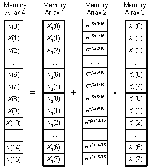
Figure 1: 16-point DFT using two 8-point FFTs.

We describe the above process, algebraically, as

X(k) = X₀(k) + e^-j2πk/16 · X₁(k) (1)

and

X(k + 8) = X₀(k) + e^{-j2π(k+8)/16} · X₁(k) (1')

for k in the range 0 ≤ k ≤ 7.

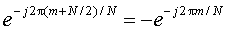
Notice that we did nothing to reduce the size of Memory Array 2 due to redundancies in the complex exponential sequence e^-j2πm/N. As it turns out, for an N-point DFT, only N/4 complex values need be stored in Memory Array 2. The reason for this is because

(2)

which involves a simple sign change on e^-j2πm/N. In addition,

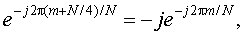(2')

which is merely swapping the real and imaginary parts of e^-j2πm/N plus a sign change of the resulting imaginary part.  So Eqs. (2) and (2') tell us that only the values e^-j2πm/N for 0 ≤ m ≤ N/4-1 need be stored in Memory Array 2. With that reduced storage idea aside, to be clear regarding exactly what computations are needed for our 'multiple-FFTs' technique we leave Memory Array 2 unchanged from what is in Figure 1.

The neat part of this 'multiple-FFTs' scheme is that our DFT length, N, is not restricted to be an integer power of two. We can use computationally efficient radix-2 FFTs to compute DFTs whose lengths are any integer multiple of an integer power of two. For example, we can compute an N = 24-point DFT using three 8-point FFTs. To do so, we perform an 8-point FFT on the x(n) samples, where n = 0, 3, 6, ..., 21, to obtain X₀(k). Next we compute an 8-point FFT on the x(n) samples, where n = 1, 4, 7, ..., 22 to yield X₁(k). And then we perform an 8-point FFT on the x(n) samples, where n = 2, 5, 8, ..., 23, to obtain an X₂(k) sequence. Finally we compute our desired 24-point DFT results using

X(k) = X₀(k) + e^-j2πk/24 · X₁(k) + e^-j2π(2k)/24 · X₂(k) (3)

X(k + 8) = X₀(k) + e^{-j2π(k+8)/24} · X₁(k) + e^{-j2π[2(k+8)]/24} · X₂(k) (3')

and

X(k + 16) = X₀(k) + e^{-j2π(k+16)/24} · X₁(k) + e^{-j2π[2(k+16)]/24} · X₂(k). (3'')

for k in the range 0 ≤ k ≤ 7. The memory-array depiction of this process is shown in Figure 2, with our final 24-point DFT results residing in Memory Array 6. Memory Array 2 contains N = 24 samples of one cycle of the complex exponential e^-j2πm/24, where 0 ≤ m ≤ 23. Memory Array 4 contains 24 samples of two cycles of the complex exponential e^-j2π(2m)/24.

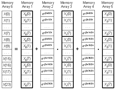
Figure 2 24-point DFT using three 8-point FFTs.

To conclude this blog, we mention that the larger the size of the FFTs the more computationally efficient is this 'multiple-FFTs' spectrum analysis technique. This behavior is illustrated in Figure 3 where we show the number of complex multiplies required by the 'multiple-FFTs' algorithm versus the desired DFT size (N). The top bold curve is the number of complex multiplies required by the standard (inefficient) DFT algorithm, and the bottom dashed curve is the number of complex multiplies required by a single N-point radix-2 FFT. The curves in the center of the figure show the number of complex multiplies required by the 'multiple-FFTs' algorithm when various FFT sizes (P) are used to compute an N-point DFT.

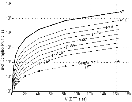
Figure 3 Number of complex multiplies versus N.

kaushik l wrote:

Rick Lyons wrote:

franchouze wrote:

Rick Lyons wrote:

dnevins wrote:

Rick Lyons wrote:

dnevins wrote:

Rick Lyons wrote:

mahesh663 wrote: