


Identifying Chirp Rate
Consider again the Fourier transform of a complex Gaussian in (10.27):
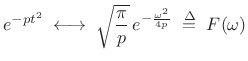 |
(11.33) |
Setting
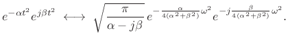 |
(11.34) |
The log magnitude Fourier transform is given by
| (11.35) |
and the phase is
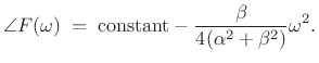 |
(11.36) |
Note that both log-magnitude and (unwrapped) phase are parabolas in
In practice, it is simple to estimate the curvature at a spectral peak using parabolic interpolation:
![\begin{eqnarray*}
c_m &\isdef & \frac{d^2}{d\omega^2} \ln\vert F(\omega)\vert \eqsp - \frac{\alpha}{2(\alpha^2+\beta^2)}\\ [5pt]
c_p &\isdef & \frac{d^2}{d\omega^2} \angle F(\omega) \eqsp - \frac{\beta}{2(\alpha^2+\beta^2)}
\end{eqnarray*}](http://www.dsprelated.com/josimages_new/sasp2/img1886.png)
We can write

Note that the window ``amplitude-rate'' ![]() is always positive.
The ``chirp rate''
is always positive.
The ``chirp rate'' ![]() may be positive (increasing frequency) or
negative (downgoing chirps). For purposes of chirp-rate estimation,
there is no need to find the true spectral peak because the curvature
is the same for all
may be positive (increasing frequency) or
negative (downgoing chirps). For purposes of chirp-rate estimation,
there is no need to find the true spectral peak because the curvature
is the same for all ![]() . However, curvature estimates are
generally more reliable near spectral peaks, where the signal-to-noise
ratio is typically maximum.
In practice, we can form an estimate of
. However, curvature estimates are
generally more reliable near spectral peaks, where the signal-to-noise
ratio is typically maximum.
In practice, we can form an estimate of ![]() from the known FFT
analysis window (typically ``close to Gaussian'').
from the known FFT
analysis window (typically ``close to Gaussian'').
Chirplet Frequency-Rate Estimation
The chirp rate ![]() may be estimated from the relation
may be estimated from the relation
![]() as follows:
as follows:
- Let
 denote the measured (or known) curvature at the
midpoint of the analysis window
denote the measured (or known) curvature at the
midpoint of the analysis window  .
.
- Let
![$ [c_m]$](http://www.dsprelated.com/josimages_new/sasp2/img1890.png) and
and ![$ [c_p]$](http://www.dsprelated.com/josimages_new/sasp2/img1891.png) denote weighted
averages of the measured curvatures
denote weighted
averages of the measured curvatures  and
and  along the log-magnitude and phase of a spectral peak,
respectively.
along the log-magnitude and phase of a spectral peak,
respectively.
- Then the chirp-rate
 estimate may be estimated from the
spectral peak by
estimate may be estimated from the
spectral peak by
![$\displaystyle \zbox {{\hat \beta}\isdefs {\hat \alpha}\frac{[c_p]}{[c_m]}}
$](http://www.dsprelated.com/josimages_new/sasp2/img1894.png)
Simulation Results
![\includegraphics[width=\twidth]{eps/gwchirp}](http://www.dsprelated.com/josimages_new/sasp2/img1895.png)
Figure 10.24 shows the waveform of a Gaussian-windowed chirp (``chirplet'') generated by the following matlab code:
fs = 8000;
x = chirp([0:1/fs:0.1],1000,1,2000);
M = length(x);
n=(-(M-1)/2:(M-1)/2)';
w = exp(-n.*n./(2*sigma.*sigma));
xw = w(:) .* x(:);
Figure 10.25 shows the same chirplet in a time-frequency plot. Figure 10.26 shows the spectrum of the example chirplet. Note the parabolic fits to dB magnitude and unwrapped phase. We see that phase modeling is most accurate where magnitude is substantial. If the signal were not truncated in the time domain, the parabolic fits would be perfect. Figure 10.27 shows the spectrum of a Gaussian-windowed chirp in which frequency decreases from 1 kHz to 500 Hz. Note how the curvature of the phase at the peak has changed sign.
![\includegraphics[width=\twidth]{eps/gwchirpsgC}](http://www.dsprelated.com/josimages_new/sasp2/img1896.png)
![\includegraphics[width=\twidth]{eps/gwchirpxform}](http://www.dsprelated.com/josimages_new/sasp2/img1897.png)
![\includegraphics[width=\twidth]{eps/gwchirpdownxform}](http://www.dsprelated.com/josimages_new/sasp2/img1898.png)
![\includegraphics[width=\twidth,height=3in]{eps/gwchirpshort}](http://www.dsprelated.com/josimages_new/sasp2/img1899.png)
![\includegraphics[width=\twidth]{eps/gwchirpshortxform}](http://www.dsprelated.com/josimages_new/sasp2/img1900.png)
Next Section:
Audio Filter Banks
Previous Section:
Modulated Gaussian-Windowed Chirp


