


Implications of Linear-Time-Invariance
Using the basic properties of linearity and time-invariance, we will derive the convolution representation which gives an algorithm for implementing the filter directly in terms of its impulse response. In other words,
 |
The convolution formula plays the role of the difference equation when the impulse response is used in place of the difference-equation coefficients as a filter representation. In fact, we will find that, for FIR filters (nonrecursive, i.e., no feedback), the difference equation and convolution representation are essentially the same thing. For recursive filters, one can think of the convolution representation as the difference equation with all feedback terms ``expanded'' to an infinite number of feedforward terms.
An outline of the derivation of the convolution formula is as follows:
Any signal ![]() may be regarded as a superposition of impulses at
various amplitudes and arrival times, i.e., each sample of
may be regarded as a superposition of impulses at
various amplitudes and arrival times, i.e., each sample of ![]() is
regarded as an impulse with amplitude
is
regarded as an impulse with amplitude ![]() and delay
and delay ![]() . We can
write this mathematically as
. We can
write this mathematically as
![]() . By the
superposition principle for LTI filters, the filter output is simply
the superposition of impulse
responses
. By the
superposition principle for LTI filters, the filter output is simply
the superposition of impulse
responses ![]() , each having a scale factor and time-shift given by
the amplitude and time-shift of the corresponding input impulse.
Thus, the sample
, each having a scale factor and time-shift given by
the amplitude and time-shift of the corresponding input impulse.
Thus, the sample ![]() contributes the signal
contributes the signal
![]() to
the convolution output, and the total output is the sum of such
contributions, by superposition. This is the heart of LTI filtering.
to
the convolution output, and the total output is the sum of such
contributions, by superposition. This is the heart of LTI filtering.
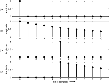
Before proceeding to the general case, let's look at a simple example
with pictures. If an impulse strikes at time ![]() rather than at
time
rather than at
time ![]() , this is represented by writing
, this is represented by writing
![]() . A
picture of this delayed impulse is given in Fig.5.2c. When
. A
picture of this delayed impulse is given in Fig.5.2c. When
![]() is fed to a time-invariant filter, the output will be
the impulse response
is fed to a time-invariant filter, the output will be
the impulse response ![]() delayed by 5 samples, or
delayed by 5 samples, or ![]() . Figure 5.2d shows the response of the example filter of
Eq.
. Figure 5.2d shows the response of the example filter of
Eq.![]() (5.3) to the delayed impulse
(5.3) to the delayed impulse
![]() .
.
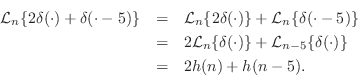
In the general case, for time-invariant filters we may write
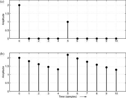
If two impulses arrive at the filter input, the first at time ![]() ,
say, and the second at time
,
say, and the second at time ![]() , then this input may be expressed
as
, then this input may be expressed
as
![]() . If, in addition, the amplitude of the
first impulse is 2, while the second impulse has an amplitude of 1,
then the input may be written as
. If, in addition, the amplitude of the
first impulse is 2, while the second impulse has an amplitude of 1,
then the input may be written as
![]() . In
this case, using linearity as well as time-invariance, the
response of the general LTI filter to this input may be expressed as
. In
this case, using linearity as well as time-invariance, the
response of the general LTI filter to this input may be expressed as
For the example filter of Eq.![]() (5.3), given the input
(5.3), given the input
![]() (pictured in Fig.5.3a),
the output may be computed by scaling, shifting, and adding together
copies of the impulse response
(pictured in Fig.5.3a),
the output may be computed by scaling, shifting, and adding together
copies of the impulse response ![]() . That is, taking the impulse
response in Fig.5.2b, multiplying it by 2, and adding it to the
delayed impulse response in Fig.5.2d, we obtain the output
shown in Fig.5.3b. Thus, a weighted sum of impulses produces
the same weighted sum of impulse responses.
. That is, taking the impulse
response in Fig.5.2b, multiplying it by 2, and adding it to the
delayed impulse response in Fig.5.2d, we obtain the output
shown in Fig.5.3b. Thus, a weighted sum of impulses produces
the same weighted sum of impulse responses.
 |
Next Section:
Convolution Representation
Previous Section:
Impulse Response Example


