First-Order Parallel Sections

Figure 3.13 shows the impulse response of the real one-pole section

$\displaystyle H_1(z) = \frac{0.1657}{1 + 0.9z^{-1}},$

and Fig.3.14 shows its frequency response, computed using the matlab utility myfreqz listed in §7.5.1. (Both Matlab and Octave have compatible utilities freqz, which serve the same purpose.) Note that the sampling rate is set to 1, and the frequency axis goes from 0 Hz all the way to the sampling rate, which is appropriate for complex filters (as we will soon see). Since real filters have Hermitian frequency responses (i.e., an even amplitude response and odd phase response), they may be plotted from 0 Hz to half the sampling rate without loss of information.

**Figure 3.13:** Impulse response of section 1 of the example filter.
$\includegraphics[width=\textwidth]{eps/arir1}$

**Figure 3.14:** Frequency response of section 1 of the example filter.
$\includegraphics[width=\textwidth]{eps/arfr1}$

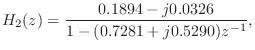
Figure 3.15 shows the impulse response of the complex one-pole section

$\displaystyle H_2(z) = \frac{0.1894 - j 0.0326}{1 - (0.7281 + j 0.5290)z^{-1}},$

and Fig.3.16 shows the corresponding frequency response.

**Figure 3.15:** Impulse response of complex one-pole section 2 of the full partial-fraction-expansion of the example filter.
$\includegraphics[width=\textwidth]{eps/arcir2}$

**Figure 3.16:** Frequency response of complex one-pole section 2.
$\includegraphics[width=\textwidth]{eps/arcfr2}$

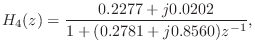
The complex-conjugate section,

$\displaystyle H_3(z) = \frac{0.1894 + j 0.0326}{1 - (0.7281 - j 0.5290)z^{-1}},$

is of course quite similar, and is shown in Figures 3.17 and 3.18.

**Figure 3.17:** Impulse response of complex one-pole section 3 of the full partial-fraction-expansion of the example filter.
$\includegraphics[width=\textwidth]{eps/arcir3}$

**Figure 3.18:** Frequency response of complex one-pole section 3.
$\includegraphics[width=\textwidth]{eps/arcfr3}$

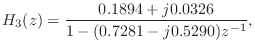
Figure 3.19 shows the impulse response of the complex one-pole section

$\displaystyle H_4(z) = \frac{0.2277 + j 0.0202}{1 + (0.2781 + j 0.8560)z^{-1}},$

and Fig.3.20 shows its frequency response. Its complex-conjugate counterpart,

, is not shown since it is analogous to

in relation to

**Figure 3.19:** Impulse response of complex one-pole section 4 of the full partial-fraction-expansion of the example filter.
$\includegraphics[width=\textwidth]{eps/arcir4}$

**Figure 3.20:** Frequency response of complex one-pole section 4.
$\includegraphics[width=\textwidth]{eps/arcfr4}$

Order a Hardcopy of Introduction to Digital Filters

Previous: Alternative Realizations
Next: Parallel, Real, Second-Order Sections

written by Julius Orion Smith III
Julius Smith's background is in electrical engineering (BS Rice 1975, PhD Stanford 1983). He is presently Professor of Music and Associate Professor (by courtesy) of Electrical Engineering at Stanford's Center for Computer Research in Music and Acoustics (CCRMA), teaching courses and pursuing research related to signal processing applied to music and audio systems. See http://ccrma.stanford.edu/~jos/ for details.

Sign in

Search Online Books

Free Online Books

Ads

Chapters

Introduction to Digital Filters
    Analysis of a Digital Comb Filter
       Alternative Realizations
          First-Order Parallel Sections