


Poles and Zeros of the Cepstrum
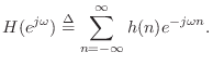
The complex cepstrum of a sequence ![]() is typically defined
as the inverse Fourier transform of its log spectrum
[60]
is typically defined
as the inverse Fourier transform of its log spectrum
[60]
![$\displaystyle {\tilde h}(n)\isdef \frac{1}{2\pi}\int_{-\pi}^\pi \ln[H(e^{j\omega})] e^{j\omega n}d\omega,
$](http://www.dsprelated.com/josimages_new/filters/img1095.png)
From Eq.![]() (8.2), the log z transform can be written in terms of the
factored form as
(8.2), the log z transform can be written in terms of the
factored form as
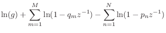
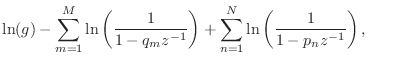
where
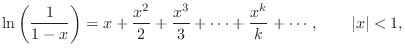
Since the region of convergence of the z transform must include the unit
circle (where the spectrum (DTFT) is defined), we see that the
Maclaurin expansion gives us the inverse z transform of all terms of
Eq.![]() (8.9) corresponding to poles and zeros inside the unit
circle of the
(8.9) corresponding to poles and zeros inside the unit
circle of the ![]() plane. Since the poles must be inside the unit
circle anyway for stability, this restriction is normally not binding
for the poles. However, zeros outside the unit circle--so-called
``non-minimum-phase zeros''--are used quite often in practice.
plane. Since the poles must be inside the unit
circle anyway for stability, this restriction is normally not binding
for the poles. However, zeros outside the unit circle--so-called
``non-minimum-phase zeros''--are used quite often in practice.
For a zero (or pole) outside the unit circle, we may rewrite the
corresponding term of Eq.![]() (8.9) as
(8.9) as
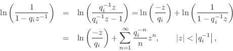
where we used the Maclaurin series expansion for
![]() once
again with the region of convergence including the unit circle. The
infinite sum in this expansion is now the bilateral z transform of an
anticausal sequence, as discussed in §8.7. That is,
the time-domain sequence is zero for nonnegative times (
once
again with the region of convergence including the unit circle. The
infinite sum in this expansion is now the bilateral z transform of an
anticausal sequence, as discussed in §8.7. That is,
the time-domain sequence is zero for nonnegative times (![]() ) and
the sequence decays in the direction of time minus-infinity. The
factored-out terms
) and
the sequence decays in the direction of time minus-infinity. The
factored-out terms ![]() and
and ![]() , for all poles and zeros
outside the unit circle, can be collected together and associated with
the overall gain factor
, for all poles and zeros
outside the unit circle, can be collected together and associated with
the overall gain factor ![]() in Eq.
in Eq.![]() (8.9), resulting in a modified
scaling and time-shift for the original sequence
(8.9), resulting in a modified
scaling and time-shift for the original sequence ![]() which can be
dealt with separately [60].
which can be
dealt with separately [60].
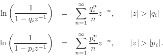
When all poles and zeros are inside the unit circle, the complex cepstrum is causal and can be expressed simply in terms of the filter poles and zeros as
![$\displaystyle {\tilde h}(n) = \left\{\begin{array}{ll}
\ln(g), & n=0 \\ [5pt]
\...
...ystyle\sum_{k=1}^M \frac{q_k^n}{n}, & n=1,2,3,\ldots\,, \\
\end{array}\right.
$](http://www.dsprelated.com/josimages_new/filters/img1115.png)
In summary, each stable pole contributes a positive decaying
exponential (weighted by ![]() ) to the complex cepstrum, while each
zero inside the unit circle contributes a negative
weighted-exponential of the same type. The decaying exponentials
start at time 1 and have unit amplitude (ignoring the
) to the complex cepstrum, while each
zero inside the unit circle contributes a negative
weighted-exponential of the same type. The decaying exponentials
start at time 1 and have unit amplitude (ignoring the ![]() weighting)
in the sense that extrapolating them to time 0 (without the
weighting)
in the sense that extrapolating them to time 0 (without the ![]() weighting) would use the values
weighting) would use the values ![]() and
and
![]() . The
decay rates are faster when the poles and zeros are well inside the
unit circle, but cannot decay slower than
. The
decay rates are faster when the poles and zeros are well inside the
unit circle, but cannot decay slower than ![]() .
.
On the other hand, poles and zeros outside the unit circle contribute anticausal exponentials to the complex cepstrum, negative for the poles and positive for the zeros.
Next Section:
Conversion to Minimum Phase
Previous Section:
Unstable Poles--Unit Circle Viewpoint


