


Signal Metrics
This section defines some useful functions of signals (vectors).
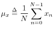
The mean of a
signal ![]() (more precisely the ``sample mean'') is defined as the
average value of its samples:5.5
(more precisely the ``sample mean'') is defined as the
average value of its samples:5.5
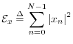
The total energy
of a signal ![]() is defined as the sum of squared moduli:
is defined as the sum of squared moduli:
In physics, energy (the ``ability to do work'') and work are in units
of ``force times distance,'' ``mass times velocity squared,'' or other
equivalent combinations of units.5.6 In digital signal processing, physical units are routinely
discarded, and signals are renormalized whenever convenient.
Therefore,
![]() is defined above without regard for constant
scale factors such as ``wave impedance'' or the sampling interval
is defined above without regard for constant
scale factors such as ``wave impedance'' or the sampling interval ![]() .
.
The average power of a signal ![]() is defined as the energy
per sample:
is defined as the energy
per sample:
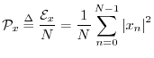
Power is always in physical units of energy per unit time. It therefore makes sense to define the average signal power as the total signal energy divided by its length. We normally work with signals which are functions of time. However, if the signal happens instead to be a function of distance (e.g., samples of displacement along a vibrating string), then the ``power'' as defined here still has the interpretation of a spatial energy density. Power, in contrast, is a temporal energy density.
The root mean square (RMS) level of a signal ![]() is simply
is simply
![]() . However, note that in practice (especially in audio
work) an RMS level is typically computed after subtracting out any
nonzero mean value.
. However, note that in practice (especially in audio
work) an RMS level is typically computed after subtracting out any
nonzero mean value.
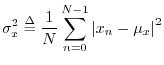
The variance (more precisely the sample variance) of the
signal ![]() is defined as the power of the signal with its mean
removed:5.7
is defined as the power of the signal with its mean
removed:5.7
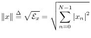
The norm (more specifically, the ![]() norm, or
Euclidean norm) of a signal
norm, or
Euclidean norm) of a signal ![]() is defined as the square root
of its total energy:
is defined as the square root
of its total energy:
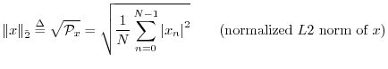
Other Lp Norms
Since our main norm is the square root of a sum of squares,
We could equally well have chosen a normalized ![]() norm:
norm:
More generally, the (unnormalized) ![]() norm of
norm of
![]() is defined as
is defined as
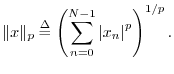
 : The
: The  , ``absolute value,'' or ``city block'' norm.
 : The
: The  , ``Euclidean,'' ``root energy,'' or ``least squares'' norm.
 : The
: The
 , ``Chebyshev,'' ``supremum,'' ``minimax,''
or ``uniform'' norm.
, ``Chebyshev,'' ``supremum,'' ``minimax,''
or ``uniform'' norm.
Norm Properties
There are many other possible choices of norm. To qualify as a norm
on ![]() , a real-valued signal-function
, a real-valued signal-function
![]() must
satisfy the following three properties:
must
satisfy the following three properties:
-
 , with

-
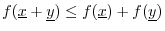
-
 ,
,

Banach Spaces
Mathematically, what we are working with so far is called a
Banach space, which is a normed linear vector space. To
summarize, we defined our vectors as any list of ![]() real or complex
numbers which we interpret as coordinates in the
real or complex
numbers which we interpret as coordinates in the ![]() -dimensional
vector space. We also defined vector addition (§5.3) and
scalar multiplication (§5.5) in the obvious way. To have
a linear vector space (§5.7), it must be closed
under vector addition and scalar multiplication (linear
combinations). I.e., given any two vectors
-dimensional
vector space. We also defined vector addition (§5.3) and
scalar multiplication (§5.5) in the obvious way. To have
a linear vector space (§5.7), it must be closed
under vector addition and scalar multiplication (linear
combinations). I.e., given any two vectors
![]() and
and
![]() from the vector space, and given any two scalars
from the vector space, and given any two scalars
![]() and
and
![]() from the field of scalars
from the field of scalars ![]() , the linear
combination
, the linear
combination
![]() must also be in the space. Since
we have used the field of complex numbers
must also be in the space. Since
we have used the field of complex numbers ![]() (or real numbers
(or real numbers
![]() ) to define both our scalars and our vector components, we
have the necessary closure properties so that any linear combination
of vectors from
) to define both our scalars and our vector components, we
have the necessary closure properties so that any linear combination
of vectors from ![]() lies in
lies in ![]() . Finally, the definition of a
norm (any norm) elevates a vector space to a Banach space.
. Finally, the definition of a
norm (any norm) elevates a vector space to a Banach space.
Next Section:
The Inner Product
Previous Section:
Linear Vector Space


