


Ideal Vibrating String
![\includegraphics[scale=0.9]{eps/FphysicalstringCopy}](http://www.dsprelated.com/josimages_new/pasp/img1307.png)
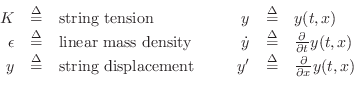
The ideal vibrating string is depicted in Fig.6.1. It is assumed to be perfectly flexible and elastic. Once ``plucked,'' it will vibrate forever in one plane as an energy conserving system. The mathematical theory of string vibration is considered in §B.6 and Appendix C. For present purposes, we only need some basic definitions and results.
Wave Equation
The wave equation for the ideal vibrating string may be written as
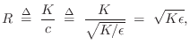
where we define the following notation:
 |
As discussed in Chapter 1, the wave equation in this form can be interpreted as a statement of Newton's second law,
Wave Equation Applications
The ideal-string wave equation applies to any perfectly elastic medium which is displaced along one dimension. For example, the air column of a clarinet or organ pipe can be modeled using the one-dimensional wave equation by substituting air-pressure deviation for string displacement, and longitudinal volume velocity for transverse string velocity. We refer to the general class of such media as one-dimensional waveguides. Extensions to two and three dimensions (and more, for the mathematically curious), are also possible (see §C.14) [518,520,55].
For a physical string model, at least three coupled waveguide models should be considered. Two correspond to transverse-wave vibrations in the horizontal and vertical planes (two polarizations of planar vibration); the third corresponds to longitudinal waves. For bowed strings, torsional waves should also be considered, since they affect bow-string dynamics [308,421]. In the piano, for key ranges in which the hammer strikes three strings simultaneously, nine coupled waveguides are required per key for a complete simulation (not including torsional waves); however, in a practical, high-quality, virtual piano, one waveguide per coupled string (modeling only the vertical, transverse plane) suffices quite well [42,43]. It is difficult to get by with fewer than the correct number of strings, however, because their detuning determines the entire amplitude envelope as well as beating and aftersound effects [543].
Traveling-Wave Solution
It can be readily checked (see §C.3 for details) that the lossless 1D wave equation

Note that we have
Sampled Traveling-Wave Solution
As discussed in more detail in Appendix C, the continuous traveling-wave
solution to the wave equation given in Eq.![]() (6.2) can be sampled
to yield
(6.2) can be sampled
to yield
where
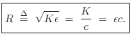
Wave Impedance
A concept of high practical utility is that of wave impedance, defined for vibrating strings as force divided by velocity. As derived in §C.7.2, the relevant force quantity in this case is minus the string tension times the string slope:
| (7.4) |
Physically, this can be regarded as the transverse force acting to the right on the string in the vertical direction. (Only transverse vibration is being considered.) In other words, the vertical component of a negative string slope pulls ``up'' on the segment of string to the right, and ``up'' is the positive direction for displacement, velocity, and now force. The traveling-wave decomposition of the force into force waves is thus given by (see §C.7.2 for a more detailed derivation)7.2

where we have defined the new notation
![]() for transverse velocity, and
for transverse velocity, and
The wave impedance simply relates force and velocity traveling waves:
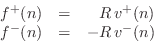
These relations may be called Ohm's law for traveling waves. Thus, in a traveling wave, force is always in phase with velocity (considering the minus sign in the left-going case to be associated with the direction of travel rather than a
The results of this section are derived in more detail in
Appendix C. However, all we need in practice for now are the
important Ohm's law relations for traveling-wave components given in
Eq.![]() (6.6).
(6.6).
Next Section:
Ideal Acoustic Tube
Previous Section:
The Leslie


