


Kaiser Window
Jim Kaiser discovered a simple approximation to the DPSS window based upon Bessel functions [115], generally known as the Kaiser window (or Kaiser-Bessel window).
Definition:
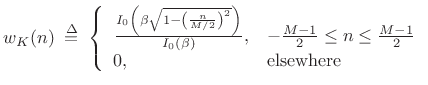 |
(4.39) |
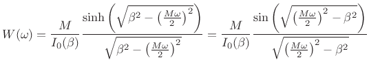
Window transform:
The Fourier transform of the Kaiser window ![]() (where
(where ![]() is
treated as continuous) is given by4.11
is
treated as continuous) is given by4.11
 |
(4.40) |
where
![$\displaystyle I_0(x) \isdefs \sum_{k=0}^{\infty} \left[ \frac{\left(\frac{x}{2}\right)^k}{k!} \right]^2
$](http://www.dsprelated.com/josimages_new/sasp2/img489.png)
Notes:
- Reduces to rectangular window for

- Asymptotic roll-off is 6 dB/octave
- First null in window transform is at

- Time-bandwidth product
 radians
if bandwidths are measured from 0 to positive band-limit
radians
if bandwidths are measured from 0 to positive band-limit
- Full time-bandwidth product
 radians
when frequency bandwidth is defined as main-lobe width
out to first null
radians
when frequency bandwidth is defined as main-lobe width
out to first null
- Sometimes the Kaiser window is parametrized by
 , where

(4.42)
Kaiser Window Beta Parameter
The ![]() parameter of the Kaiser window provides a convenient
continuous control over the fundamental window trade-off between
side-lobe level and main-lobe width. Larger
parameter of the Kaiser window provides a convenient
continuous control over the fundamental window trade-off between
side-lobe level and main-lobe width. Larger ![]() values give lower
side-lobe levels, but at the price of a wider main lobe. As discussed
in §5.4.1, widening the main lobe reduces
frequency resolution when the window is used for spectrum
analysis. As explored in Chapter 9, reducing the side lobes reduces ``channel cross
talk'' in an FFT-based filter-bank implementation.
values give lower
side-lobe levels, but at the price of a wider main lobe. As discussed
in §5.4.1, widening the main lobe reduces
frequency resolution when the window is used for spectrum
analysis. As explored in Chapter 9, reducing the side lobes reduces ``channel cross
talk'' in an FFT-based filter-bank implementation.
The Kaiser beta parameter can be interpreted as 1/4 of the
``time-bandwidth product''
![]() of the window
in radians (seconds times radians-per-second).4.13 Sometimes the Kaiser window is
parametrized by
of the window
in radians (seconds times radians-per-second).4.13 Sometimes the Kaiser window is
parametrized by
 instead of
 ![]() . The
. The
![]() parameter is therefore half the window's time-bandwidth
product
parameter is therefore half the window's time-bandwidth
product
![]() in cycles (seconds times
cycles-per-second).
in cycles (seconds times
cycles-per-second).
Kaiser Windows and Transforms
Figure 3.24 plots the Kaiser window and its transform for
![]() . Note how increasing
. Note how increasing ![]() causes the
side-lobes to fall away from the main lobe. The curvature at the main
lobe peak also decreases somewhat.
causes the
side-lobes to fall away from the main lobe. The curvature at the main
lobe peak also decreases somewhat.
![\includegraphics[width=\twidth]{eps/kaiser123}](http://www.dsprelated.com/josimages_new/sasp2/img499.png)
Figure 3.25 shows a plot of the Kaiser window
for various values of
![]() . Note that for
. Note that for ![]() , the
Kaiser window reduces to the rectangular window.
, the
Kaiser window reduces to the rectangular window.
![\includegraphics[width=\twidth]{eps/KaiserTBetas}](http://www.dsprelated.com/josimages_new/sasp2/img501.png)
Figure 3.26 shows a plot of the Kaiser window
transforms for
![]() . For
. For ![]() (top plot),
we see the dB magnitude of the aliased sinc function. As
(top plot),
we see the dB magnitude of the aliased sinc function. As ![]() increases the main-lobe widens and the side lobes go lower, reaching
almost 50 dB down for
increases the main-lobe widens and the side lobes go lower, reaching
almost 50 dB down for ![]() .
.
![\includegraphics[width=\twidth]{eps/KaiserFBetas}](http://www.dsprelated.com/josimages_new/sasp2/img504.png)
Figure 3.27 shows the effect of increasing window length
for the Kaiser window. The window lengths are
![]() from the top to the bottom plot. As with all windows, increasing the
length decreases the main-lobe width, while the side-lobe level
remains essentially unchanged.
from the top to the bottom plot. As with all windows, increasing the
length decreases the main-lobe width, while the side-lobe level
remains essentially unchanged.
![\includegraphics[width=\twidth]{eps/KaiserFLengths}](http://www.dsprelated.com/josimages_new/sasp2/img506.png)
Figure 3.28 shows a plot of the Kaiser window side-lobe level
for various values of
![]() . For
. For
![]() , the Kaiser window reduces to the rectangular window, and we
expect the side-lobe level to be about 13 dB below the main lobe
(upper-lefthand corner of Fig.3.28). As
, the Kaiser window reduces to the rectangular window, and we
expect the side-lobe level to be about 13 dB below the main lobe
(upper-lefthand corner of Fig.3.28). As
![]() increases, the dB side-lobe level reduces approximately linearly with
main-lobe width increase (approximately a 25 dB drop in side-lobe
level for each main-lobe width increase by one sinc-main-lobe).
increases, the dB side-lobe level reduces approximately linearly with
main-lobe width increase (approximately a 25 dB drop in side-lobe
level for each main-lobe width increase by one sinc-main-lobe).
![\includegraphics[width=\twidth]{eps/kaiserBeta}](http://www.dsprelated.com/josimages_new/sasp2/img508.png)
Minimum Frequency Separation vs. Window Length
The requirements on window length for resolving closely tuned
sinusoids was discussed in §5.5.2. This section considers
this issue for the Kaiser window. Table 3.1 lists the ![]() parameter required for a Kaiser window to resolve equal-amplitude
sinusoids with a frequency spacing of
parameter required for a Kaiser window to resolve equal-amplitude
sinusoids with a frequency spacing of
![]() rad/sample
[1, Table 8-9]. Recall from §3.9 that
rad/sample
[1, Table 8-9]. Recall from §3.9 that
![]() can be interpreted as half of the time-bandwidth of the
window (in cycles).
can be interpreted as half of the time-bandwidth of the
window (in cycles).
|
Kaiser and DPSS Windows Compared
Figure 3.29 shows an overlay of DPSS and Kaiser windows
for some different ![]() values. In all cases, the window length
was
values. In all cases, the window length
was ![]() . Note how the two windows become more similar as
. Note how the two windows become more similar as ![]() increases. The Matlab for computing the windows is as follows:
increases. The Matlab for computing the windows is as follows:
  w1 = dpss(M,alpha,1);    % discrete prolate spheroidal seq.
  w2 = kaiser(M,alpha*pi); % corresponding kaiser window
![\includegraphics[width=\twidth]{eps/dpsstest}](http://www.dsprelated.com/josimages_new/sasp2/img515.png)
The following Matlab comparison of the DPSS and Kaiser windows
illustrates the interpretation of ![]() as the bin number of the
edge of the critically sampled window main lobe, i.e., when the DFT
length equals the window length:
as the bin number of the
edge of the critically sampled window main lobe, i.e., when the DFT
length equals the window length:
format long;
M=17;
alpha=5;
abs(fft([ dpss(M,alpha,1), kaiser(M,pi*alpha)/2]))
ans =
   2.82707022360190   2.50908747431366
   2.00652719015325   1.92930705688346
   0.68469697658600   0.85272343521683
   0.09415916813555   0.19546670371747
   0.00311639169878   0.01773139505899
   0.00000050775691   0.00022611995322
   0.00000003737279   0.00000123787805
   0.00000000262633   0.00000066206722
   0.00000007448708   0.00000034793207
   0.00000007448708   0.00000034793207
   0.00000000262633   0.00000066206722
   0.00000003737279   0.00000123787805
   0.00000050775691   0.00022611995322
   0.00311639169878   0.01773139505899
   0.09415916813555   0.19546670371747
   0.68469697658600   0.85272343521683
   2.00652719015325   1.92930705688346
Finally, Fig.3.30 shows a comparison of DPSS and Kaiser window transforms, where the DPSS window was computed using the simple method listed in §F.1.2. We see that the DPSS window has a slightly narrower main lobe and lower overall side-lobe levels, although its side lobes are higher far from the main lobe. Thus, the DPSS window has slightly better overall specifications, while Kaiser-window side lobes have a steeper roll off.
![\includegraphics[width=\twidth]{eps/dpsskaiser-fd}](http://www.dsprelated.com/josimages_new/sasp2/img516.png)
Next Section:
Dolph-Chebyshev Window
Previous Section:
Slepian or DPSS Window


