


Sample Autocorrelation
The sample autocorrelation of a sequence ![]() ,
,
![]() may be defined by
may be defined by
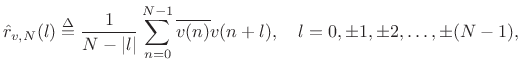
where
![$\displaystyle \left\{\begin{array}{ll} \frac{1}{N-l}\sum_{n=0}^{N-1-l}\overline{v(n)}v(n+l), & l=0,1,2,\ldots,N-1 \\ [5pt] \frac{1}{N+l}\sum_{n=-l}^{N-1}\overline{v(n)}v(n+l), & l=-1,-2,\ldots,-N+1 \\ \end{array} \right. \protect$](http://www.dsprelated.com/josimages_new/sasp2/img1111.png)
and zero for
In matlab, the sample autocorrelation of a vector x can be computed using the xcorr function.7.3
Example:
octave:1> xcorr([1 1 1 1], 'unbiased')
ans =
  1   1   1   1   1   1   1
The xcorr function also performs cross-correlation when given a second signal argument, and offers additional features with additional arguments. Say help xcorr for details.
Note that
![]() is the average of the lagged product
is the average of the lagged product
![]() over all available data. For white noise, this
average approaches zero for
over all available data. For white noise, this
average approaches zero for ![]() as the number of terms in the
average increases. That is, we must have
as the number of terms in the
average increases. That is, we must have
![$\displaystyle \hat{r}_{v,N}(l) \approx \left\{\begin{array}{ll} \hat{\sigma}_{v,N}^2, & l=0 \\ [5pt] 0, & l\neq 0 \\ \end{array} \right. \isdef \hat{\sigma}_{v,N}^2 \delta(l)$](http://www.dsprelated.com/josimages_new/sasp2/img1116.png) |
(7.8) |
where
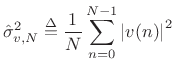 |
(7.9) |
is defined as the sample variance of
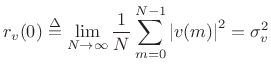
The plot in the upper left corner of Fig.6.1 shows the sample autocorrelation obtained for 32 samples of pseudorandom numbers (synthetic random numbers). (For reasons to be discussed below, the sample autocorrelation has been multiplied by a Bartlett (triangular) window.) Proceeding down the column on the left, the results of averaging many such sample autocorrelations can be seen. It is clear that the average sample autocorrelation function is approaching an impulse, as desired by definition for white noise. (The right column shows the Fourier transform of each sample autocorrelation function, which is a smoothed estimate of the power spectral density, as discussed in §6.6 below.)
![\includegraphics[width=\twidth]{eps/twhite}](http://www.dsprelated.com/josimages_new/sasp2/img1118.png)
For stationary stochastic processes ![]() , the sample autocorrelation
function
, the sample autocorrelation
function
![]() approaches the true autocorrelation function
approaches the true autocorrelation function
![]() in the limit as the number of observed samples
in the limit as the number of observed samples ![]() goes to
infinity, i.e.,
goes to
infinity, i.e.,
| (7.10) |
The true autocorrelation function of a random process is defined in Appendix C. For our purposes here, however, the above limit can be taken as the definition of the true autocorrelation function for the noise sequence
At lag ![]() , the autocorrelation function of a zero-mean random
process
, the autocorrelation function of a zero-mean random
process ![]() reduces to the variance:
reduces to the variance:
The variance can also be called the average power or mean square. The square root
Next Section:
Sample Power Spectral Density
Previous Section:
White Noise


