


An FFT-Based Equation-Error Method
The algorithm below minimizes the equation error in the frequency-domain. As a result, it can make use of the FFT for speed. This algorithm is implemented in Matlab's invfreqz() function when no iteration-count is specified. (The iteration count gives that many iterations of the Steiglitz-McBride algorithm, thus transforming equation error to output error after a few iterations. There is also a time-domain implementation of the Steiglitz-McBride algorithm called stmcb() in the Matlab Signal Processing Toolbox, which takes the desired impulse response as input.)
Given a desired spectrum
![]() at equally spaced frequencies
at equally spaced frequencies
![]() , with
, with ![]() a power of
a power of ![]() ,
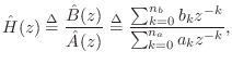
it is desired to find a rational digital
filter with
,
it is desired to find a rational digital
filter with ![]() zeros and
zeros and ![]() poles,
poles,
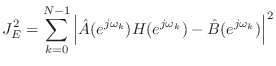
Since ![]() is a quadratic form, the solution is readily obtained by
equating the gradient to zero. An easier derivation follows from minimizing
equation error variance in the time domain and making use of the orthogonality
principle [36].
This may be viewed as a system identification problem where the
known input signal is an impulse, and the known output is the desired
impulse response. A formulation employing an arbitrary known input
is valuable for introducing complex weighting across the frequency grid,
and this general form is presented. A detailed derivation appears in
[78, Chapter 2], and here only the final algorithm is given:
is a quadratic form, the solution is readily obtained by
equating the gradient to zero. An easier derivation follows from minimizing
equation error variance in the time domain and making use of the orthogonality
principle [36].
This may be viewed as a system identification problem where the
known input signal is an impulse, and the known output is the desired
impulse response. A formulation employing an arbitrary known input
is valuable for introducing complex weighting across the frequency grid,
and this general form is presented. A detailed derivation appears in
[78, Chapter 2], and here only the final algorithm is given:
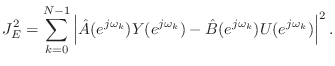
Given spectral output samples
![]() and input
samples
and input
samples
![]() , we minimize
, we minimize
Let
![]() :
:![]() denote the column vector determined
by
denote the column vector determined
by ![]() , for
, for
![]() filled in from top to bottom, and let
filled in from top to bottom, and let
![]() :
:![]() denote the size
denote the size ![]() symmetric Toeplitz matrix consisting of
symmetric Toeplitz matrix consisting of
![]() :
:![]() in its first column.
A nonsymmetric Toeplitz matrix may be specified by its first column and row,
and we use the notation
in its first column.
A nonsymmetric Toeplitz matrix may be specified by its first column and row,
and we use the notation
![]() :
:![]() :
:![]() to denote the
to denote the
![]() by
by ![]() Toeplitz matrix with left-most column
Toeplitz matrix with left-most column
![]() :
:![]() and top row
and top row
![]() :
:![]() .
The inverse Fourier transform of
.
The inverse Fourier transform of
![]() is defined as
is defined as

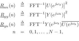
where the overbar denotes complex conjugation, and four corresponding Toeplitz matrices,
![\begin{eqnarray*}
R_{yy} &\isdef & T(\underline{R}_{yy}[0\,\mbox{:}\,{{n}_a}-1])...
...u}^T[-1\,\mbox{:}\,-{{n}_a}])\\
R_{uy} &\isdef & R_{uy}^T , \\
\end{eqnarray*}](http://www.dsprelated.com/josimages_new/filters/img2450.png)
where negative indices are to be interpreted mod ![]() , e.g.,
, e.g.,
![]() .
.
The solution is then
![$\displaystyle \hat{\theta}^\ast = \left[\begin{array}{c} \underline{\hat{B}}^\a...
...,{{n}_b}] \\ [2pt] \underline{R}_{yy}[1\,\mbox{:}\,{{n}_a}] \end{array}\right]
$](http://www.dsprelated.com/josimages_new/filters/img2452.png)
![$\displaystyle \underline{\hat{B}}^\ast \isdef \left[\begin{array}{c} \hat{b}^\a...
...t{a}^\ast _0 \\ [2pt] \vdots \\ [2pt] \hat{a}^\ast _{{n}_a}\end{array}\right],
$](http://www.dsprelated.com/josimages_new/filters/img2453.png)
Next Section:
Prony's Method
Previous Section:
Stability of Equation Error Designs


