


Showing Linearity and Time Invariance, or Not
The filter
![]() is nonlinear and time invariant. The
scaling property of linearity clearly fails since, scaling
is nonlinear and time invariant. The
scaling property of linearity clearly fails since, scaling ![]() by
by
![]() gives the output signal
gives the output signal
![]() , while
, while
![]() . The filter is time invariant, however, because delaying
. The filter is time invariant, however, because delaying ![]() by
by ![]() samples gives
samples gives ![]() which is the same as
which is the same as ![]() .
.
The filter
![]() is linear and time varying.
We can show linearity by setting the input to a linear combination of
two signals
is linear and time varying.
We can show linearity by setting the input to a linear combination of
two signals
![]() , where
, where ![]() and
and
![]() are constants:
are constants:
![\begin{eqnarray*}
n [\alpha x_1(n) + \beta x_2(n)] &+& [\alpha x_1(n-1) + \beta ...
... [n x_2(n) + x_2(n-1)]\\
&\isdef & \alpha y_1(n) + \beta y_2(n)
\end{eqnarray*}](http://www.dsprelated.com/josimages_new/filters/img469.png)
Thus, scaling and superposition are verified. The filter is
time-varying, however, since the time-shifted output is
![]() which is not the same as the filter applied
to a time-shifted input (
which is not the same as the filter applied
to a time-shifted input (
![]() ). Note that in
applying the time-invariance test, we time-shift the input signal
only, not the coefficients.
). Note that in
applying the time-invariance test, we time-shift the input signal
only, not the coefficients.
The filter ![]() , where
, where ![]() is any constant, is nonlinear
and time-invariant, in general. The condition for time invariance is
satisfied (in a degenerate way) because a constant signal equals all
shifts of itself. The constant filter is technically linear,
however, for
is any constant, is nonlinear
and time-invariant, in general. The condition for time invariance is
satisfied (in a degenerate way) because a constant signal equals all
shifts of itself. The constant filter is technically linear,
however, for ![]() , since
, since
![]() , even though the input
signal has no effect on the output signal at all.
, even though the input
signal has no effect on the output signal at all.
Any filter of the form
![]() is linear and
time-invariant. This is a special case of a sliding linear
combination (also called a running weighted sum, or
moving average when
is linear and
time-invariant. This is a special case of a sliding linear
combination (also called a running weighted sum, or
moving average when
![]() ).
All sliding linear combinations are linear,
and they are time-invariant as well when the coefficients (
).
All sliding linear combinations are linear,
and they are time-invariant as well when the coefficients (
![]() ) are constant with respect to time.
) are constant with respect to time.
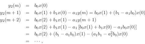
Sliding linear combinations may also include past output samples as well (feedback terms). A simple example is any filter of the form
Since linear combinations of linear combinations are linear combinations, we can use induction to show linearity and time invariance of a constant sliding linear combination including feedback terms. In the case of this example, we have, for an input signal

If the input signal is now replaced by
![]() ,
which is
,
which is ![]() delayed by
delayed by ![]() samples, then the
output
samples, then the
output ![]() is
is ![]() for
for ![]() , followed by
, followed by
or
![]() for all
for all ![]() and
and ![]() . This establishes
that each output sample from the filter of Eq.
. This establishes
that each output sample from the filter of Eq.![]() (4.7) can be expressed
as a time-invariant linear combination of present and past samples.
(4.7) can be expressed
as a time-invariant linear combination of present and past samples.
Next Section:
Nonlinear Filter Example: Dynamic Range Compression
Previous Section:
Time-Invariant Filters


