


The Simplest Lowpass Filter
Let's start with a very basic example of the generic problem at hand: understanding the effect of a digital filter on the spectrum of a digital signal. The purpose of this example is to provide motivation for the general theory discussed in later chapters.
Our example is the simplest possible low-pass filter. A low-pass
filter is one which does not affect low frequencies and rejects high
frequencies. The function giving the gain of a filter at every
frequency is called the amplitude response (or magnitude
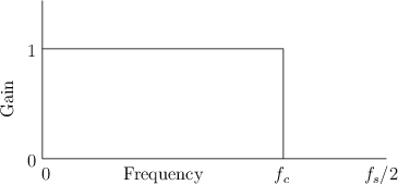
frequency response). The amplitude response of the ideal lowpass
filter is shown in Fig.1.1. Its gain is 1 in the
passband, which spans frequencies from 0 Hz to the cut-off
frequency ![]() Hz, and its gain is 0 in the stopband (all
frequencies above
Hz, and its gain is 0 in the stopband (all
frequencies above ![]() ). The output spectrum is obtained by
multiplying the input spectrum by the amplitude response of the
filter. In this way, signal components are eliminated (``stopped'')
at all frequencies above the cut-off frequency, while lower-frequency
components are ``passed'' unchanged to the output.
). The output spectrum is obtained by
multiplying the input spectrum by the amplitude response of the
filter. In this way, signal components are eliminated (``stopped'')
at all frequencies above the cut-off frequency, while lower-frequency
components are ``passed'' unchanged to the output.
Definition of the Simplest Low-Pass
The simplest (and by no means ideal) low-pass filter is given by the following difference equation:
where

It is important when working with spectra to be able to convert time
from sample-numbers, as in Eq.![]() (1.1) above, to seconds. A more
``physical'' way of writing the filter equation is
(1.1) above, to seconds. A more
``physical'' way of writing the filter equation is
To further our appreciation of this example, let's write a computer
subroutine to implement Eq.![]() (1.1). In the computer,
(1.1). In the computer, ![]() and
and
![]() are data arrays and
are data arrays and ![]() is an array index. Since sound files
may be larger than what the computer can hold in memory all at
once, we typically process the data in blocks of some reasonable
size. Therefore, the complete filtering operation consists of two
loops, one within the other. The outer loop fills the input array
is an array index. Since sound files
may be larger than what the computer can hold in memory all at
once, we typically process the data in blocks of some reasonable
size. Therefore, the complete filtering operation consists of two
loops, one within the other. The outer loop fills the input array ![]() and empties the output array
and empties the output array ![]() , while the inner loop does the actual
filtering of the
, while the inner loop does the actual
filtering of the ![]() array to produce
array to produce ![]() . Let
. Let ![]() denote the block
size (i.e., the number of samples to be processed on each iteration of
the outer loop). In the C programming language, the inner loop
of the subroutine might appear as shown in Fig.1.3. The outer
loop might read something like ``fill
denote the block
size (i.e., the number of samples to be processed on each iteration of
the outer loop). In the C programming language, the inner loop
of the subroutine might appear as shown in Fig.1.3. The outer
loop might read something like ``fill ![]() from the input file,''
``call simplp,'' and ``write out
from the input file,''
``call simplp,'' and ``write out ![]() .''
.''
/* C function implementing the simplest lowpass:
 *
 *      y(n) = x(n) + x(n-1)
 *
 */
double simplp (double *x, double *y,
               int M, double xm1)
{
  int n;
  y[0] = x[0] + xm1;
  for (n=1; n < M ; n++) {
    y[n] =  x[n]  + x[n-1];
  }
  return x[M-1];
}
|
In this implementation, the first instance of ![]() is provided as
the procedure argument xm1. That way, both
is provided as
the procedure argument xm1. That way, both ![]() and
and ![]() can
have the same array bounds (
can
have the same array bounds (
![]() ). For convenience, the
value of xm1 appropriate for the next call to
simplp is returned as the procedure's value.
). For convenience, the
value of xm1 appropriate for the next call to
simplp is returned as the procedure's value.
We may call xm1 the filter's state. It is the current
``memory'' of the filter upon calling simplp. Since this
filter has only one sample of state, it is a first order
filter. When a filter is applied to successive blocks of a signal, it
is necessary to save the filter state after processing each block.
The filter state after processing block ![]() is then the starting state
for block
is then the starting state
for block ![]() .
.
Figure 1.4 illustrates a simple main program which calls simplp. The length 10 input signal x is processed in two blocks of length 5.
/* C main program for testing simplp */
main() {
  double x[10] = {1,2,3,4,5,6,7,8,9,10};
  double y[10];

  int i;
  int N=10;
  int M=N/2; /* block size */
  double xm1 = 0;

  xm1 = simplp(x, y, M, xm1);
  xm1 = simplp(&x[M], &y[M], M, xm1);

  for (i=0;i<N;i++) {
    printf("x[%d]=%f\ty[%d]=%f\n",i,x[i],i,y[i]);
  }
  exit(0);
}
/* Output:
 *    x[0]=1.000000     y[0]=1.000000
 *    x[1]=2.000000     y[1]=3.000000
 *    x[2]=3.000000     y[2]=5.000000
 *    x[3]=4.000000     y[3]=7.000000
 *    x[4]=5.000000     y[4]=9.000000
 *    x[5]=6.000000     y[5]=11.000000
 *    x[6]=7.000000     y[6]=13.000000
 *    x[7]=8.000000     y[7]=15.000000
 *    x[8]=9.000000     y[8]=17.000000
 *    x[9]=10.000000    y[9]=19.000000
 */
|
You might suspect that since Eq.![]() (1.1) is the simplest possible
low-pass filter, it is also somehow the worst possible low-pass
filter. How bad is it? In what sense is it bad? How do we even know it
is a low-pass at all? The answers to these and related questions will
become apparent when we find the frequency response of this
filter.
(1.1) is the simplest possible
low-pass filter, it is also somehow the worst possible low-pass
filter. How bad is it? In what sense is it bad? How do we even know it
is a low-pass at all? The answers to these and related questions will
become apparent when we find the frequency response of this
filter.
Next Section:
Finding the Frequency Response
Previous Section:
Introduction


