


Plane Waves in Air
Figure B.9 shows a 2D ![]() cross-section of a snapshot (in time)
of the sinusoidal plane wave
cross-section of a snapshot (in time)
of the sinusoidal plane wave
![\includegraphics[width=\twidth]{eps/planewave}](http://www.dsprelated.com/josimages_new/pasp/img3149.png) |
Figure B.10 depicts a more mathematical schematic of a sinusoidal plane wave traveling toward the upper-right of the figure. The dotted lines indicate the crests (peak amplitude location) along the wave.
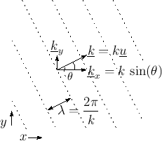
The direction of travel and spatial frequency are indicated by the
vector wavenumber
![]() , as discussed in in the following section.
, as discussed in in the following section.
Next Section:
Vector Wavenumber
Previous Section:
Air Absorption


