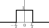
Triangular Pulse as Convolution of Two Rectangular Pulses
The 2-sample wide triangular pulse ![]() (Eq.
(Eq.![]() (4.4)) can be
expressed as a convolution of the one-sample rectangular pulse with
itself.
(4.4)) can be
expressed as a convolution of the one-sample rectangular pulse with
itself.
The one-sample rectangular pulse is shown in Fig.4.8 and may be defined analytically as

![$\displaystyle u(t) \isdef \left\{\begin{array}{ll}
1, & t\geq 0 \\ [5pt]
0, & t<0 \\
\end{array}\right..
$](http://www.dsprelated.com/josimages_new/pasp/img968.png)

Next Section:
Linear Interpolation Frequency Response
Previous Section:
Frequency Response of Linear Interpolation


