


Gaussian Moments
Gaussian Mean
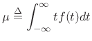
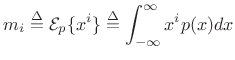
The mean of a distribution ![]() is defined as its
first-order moment:
is defined as its
first-order moment:
 |
(D.42) |
To show that the mean of the Gaussian distribution is ![]() , we may write,
letting
, we may write,
letting
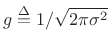 ,
,
since
![]() .
.
Gaussian Variance
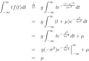
The
variance of a distribution
![]() is defined as its
second central moment:
is defined as its
second central moment:
 |
(D.43) |
where
To show that the variance of the Gaussian distribution is ![]() , we write,
letting
,
, we write,
letting
,
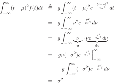
where we used integration by parts and the fact that
![]() as
as
![]() .
.
Higher Order Moments Revisited
Theorem:
The ![]() th central moment of the Gaussian pdf
th central moment of the Gaussian pdf ![]() with mean
with mean ![]() and variance
and variance ![]() is given by
is given by
![$\displaystyle m_n \isdef {\cal E}_p\{(x-\mu)^n\} = \left\{\begin{array}{ll} (n-1)!!\cdot\sigma^n, & \hbox{$n$\ even} \\ [5pt] $0$, & \hbox{$n$\ odd} \\ \end{array} \right. \protect$](http://www.dsprelated.com/josimages_new/sasp2/img2834.png)
where
Proof:
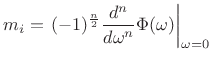
The formula can be derived by successively differentiating the
moment-generating function
![]() with respect to
with respect to ![]() and evaluating at
and evaluating at ![]() ,D.4 or by differentiating the
Gaussian integral
,D.4 or by differentiating the
Gaussian integral
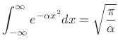 |
(D.45) |
successively with respect to
![\begin{eqnarray*}
\int_{-\infty}^\infty (-x^2) e^{-\alpha x^2} dx &=& \sqrt{\pi}(-1/2)\alpha^{-3/2}\\
\int_{-\infty}^\infty (-x^2)(-x^2) e^{-\alpha x^2} + dx &=& \sqrt{\pi}(-1/2)(-3/2)\alpha^{-5/2}\\
\vdots & & \vdots\\
\int_{-\infty}^\infty x^{2k} e^{-\alpha x^2} dx &=& \sqrt{\pi}\,[(2k-1)!!]\,2^{-k/2}\alpha^{-(k+1)/2}
\end{eqnarray*}](http://www.dsprelated.com/josimages_new/sasp2/img2843.png)
for
![]() .
Setting
.
Setting
![]() and
and ![]() , and dividing both sides by
, and dividing both sides by
![]() yields
yields
 |
(D.46) |
for
Moment Theorem
Theorem:
For a random variable ![]() ,
,
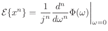 |
(D.47) |
where
 |
(D.48) |
(Note that
Proof: [201, p. 157]
Let ![]() denote the
denote the ![]() th moment of
th moment of ![]() , i.e.,
, i.e.,
 |
(D.49) |
Then
where the term-by-term integration is valid when all moments ![]() are
finite.
are
finite.
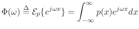
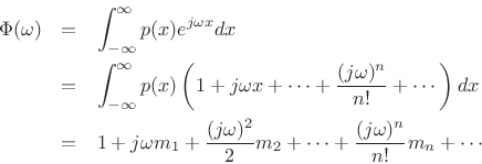
Gaussian Characteristic Function
Since the Gaussian PDF is
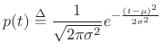 |
(D.50) |
and since the Fourier transform of
| (D.51) |
It follows that the Gaussian characteristic function is
| (D.52) |
Gaussian Central Moments
The characteristic function of a zero-mean Gaussian is
| (D.53) |
Since a zero-mean Gaussian
 |
(D.54) |
In particular,
![\begin{eqnarray*}
\Phi^\prime(\omega) &=& -\frac{1}{2}\sigma^2 2\omega\Phi(\omega)\\ [5pt]
\Phi^{\prime\prime}(\omega) &=& -\frac{1}{2}\sigma^2 2\omega\Phi^\prime(\omega)
-\frac{1}{2}\sigma^2 2\Phi(\omega)
\end{eqnarray*}](http://www.dsprelated.com/josimages_new/sasp2/img2865.png)
Since ![]() and
and
![]() , we see
, we see ![]() ,
,
![]() , as expected.
, as expected.
Next Section:
A Sum of Gaussian Random Variables is a Gaussian Random Variable
Previous Section:
Maximum Entropy Property of the Gaussian Distribution


