


Random Variable
Definition:
A random variable ![]() is defined as a real- or complex-valued
function of some random event, and is fully characterized by its
probability distribution.
is defined as a real- or complex-valued
function of some random event, and is fully characterized by its
probability distribution.
Example:
A random variable can be defined based on a coin toss by defining
numerical values for heads and tails. For example, we may assign 0 to
tails and 1 to heads. The probability distribution for this random
variable is then
![$\displaystyle \hat{p}(x) = \left\{\begin{array}{ll} \frac{1}{2}, & x = 0 \\ [5pt] \frac{1}{2}, & x = 1 \\ [5pt] 0, & \mbox{otherwise}. \\ \end{array} \right. \protect$](http://www.dsprelated.com/josimages_new/sasp2/img2624.png)
Example:
A die can be used to generate integer-valued random variables
between 1 and 6. Rolling the die provides an underlying random event.
The probability distribution of a fair die is the
discrete uniform distribution between 1 and 6. I.e.,
![$\displaystyle \hat{p}(x) = \left\{\begin{array}{ll} \frac{1}{6}, & x = 1,2,\ldots,6 \\ [5pt] 0, & \mbox{otherwise}. \\ \end{array} \right.$](http://www.dsprelated.com/josimages_new/sasp2/img2625.png) |
(C.5) |
Example:
A pair of dice can be used to generate integer-valued random
variables between 2 and 12. Rolling the dice provides an underlying
random event. The probability distribution of two fair dice is given by
![$\displaystyle \hat{p}(x) = \left\{\begin{array}{ll} \frac{x-1}{36}, & x = 2,3,\ldots,7 \\ [5pt] \frac{13-x}{36}, & x = 7,8,\ldots,12 \\ [5pt] 0, & \mbox{otherwise}. \\ \end{array} \right.$](http://www.dsprelated.com/josimages_new/sasp2/img2626.png) |
(C.6) |
This may be called a discrete triangular distribution. It can be shown to be given by the convolution of the discrete uniform distribution for one die with itself. This is a general fact for sums of random variables (the distribution of the sum equals the convolution of the component distributions).
Example:
Consider a random experiment in which a sewing needle is dropped onto
the ground from a high altitude. For each such event, the angle of
the needle with respect to north is measured. A reasonable model for
the distribution of angles (neglecting the earth's magnetic field) is
the continuous uniform distribution on ![]() , i.e., for
any real numbers
, i.e., for
any real numbers ![]() and
and ![]() in the interval
in the interval ![]() , with
, with ![]() , the probability of the needle angle falling within that interval
is
, the probability of the needle angle falling within that interval
is
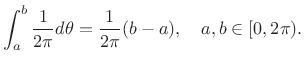 |
(C.7) |
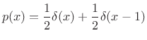
Note, however, that the probability of any single angle
![$\displaystyle p(\theta) = \left\{\begin{array}{ll} \frac{1}{2\pi}, & 0\leq \theta < 2\pi \\ [5pt] 0, & \mbox{otherwise}. \\ \end{array} \right.$](http://www.dsprelated.com/josimages_new/sasp2/img2631.png) |
(C.8) |
To calculate a probability, the PDF must be integrated over one or more intervals. As follows from Lebesgue integration theory (``measure theory''), the probability of any countably infinite set of discrete points is zero when the PDF is finite. This is because such a set of points is a ``set of measure zero'' under integration. Note that we write
 |
(C.9) |
where
Next Section:
Stochastic Process
Previous Section:
Independent Events


