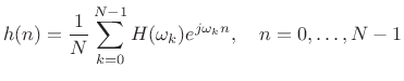
STFT with Modifications

Free Books Spectral Audio Signal Processing

FBS Fixed Modifications

Consider applying a fixed (time-invariant) filter $H(\omega_k)$ to each $X_m(\omega_k)$ before resynthesizing the signal:

$\displaystyle Y_m(\omega_k) = X_m(\omega_k)H(\omega_k)$

(10.28)

where, $H(\omega_k)$ is the sampled frequency response of a filter with impulse response

$\displaystyle h(n) = \frac{1}{N} \sum_{k=0}^{N-1} H(\omega_k) e^{j\omega_kn}, \quad n=0,\ldots,N-1$

(10.29)

Let's examine the result this has on the signal in the time domain:

$\begin{eqnarray*} y(m) &=& \frac{1}{N} \sum_{k=0}^{N-1} Y_m(\omega_k) e^{j\omega_k m} \\ &=& \frac{1}{N} \sum_{k=0}^{N-1} X_m(\omega_k)H(\omega_k) e^{j\omega_k m} \\ &=& \frac{1}{N} \sum_{k=0}^{N-1} \left\{ \sum_{n=-\infty}^\infty x(n)w(n-m)e^{-j\omega_kn} \right\} H(\omega_k) e^{j\omega_k m} \\ &=& \frac{1}{N} \sum_{n=-\infty}^\infty x(n)w(n-m) \sum_{k=0}^{N-1} H(\omega_k) e^{j\omega_k(m-n)} \\ &=& \sum_{n=-\infty}^\infty x(n) [ w(n-m) h(m-n)] \\ &=& \sum_{n=-\infty}^\infty x(n) [\tilde{w}(m-n)h(m-n)] \\ &=& (x*[\tilde{w} \cdot h])(m) \\ \end{eqnarray*}$

We see that the result is convolved with a windowed version of the impulse response . This is in contrast to the OLA technique where the result gave us a windowed filtered by without the window having any effect on the filter, provided it obeys the COLA constraint and sufficient zero padding is used to avoid time aliasing.

In other words, FBS gives

$\displaystyle y = x * [\tilde{w} \cdot h] \;\longleftrightarrow\;X \cdot [{\tilde W}\ast H]$

(10.30)

while OLA gives (for )

$\displaystyle y = x * [W(0)\cdot h] \;\longleftrightarrow\;X \cdot [W(0)\cdot H]$

(10.31)

In FBS, the analysis window smooths the filter frequency response by time-limiting the corresponding impulse response.
In OLA, the analysis window can only affect scaling.

For these reasons, FFT implementations of FIR filters normally use the Overlap-Add method.

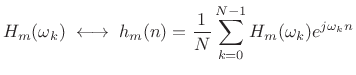
Time Varying Modifications in FBS

Consider now applying a time varying modification.

$\displaystyle Y_m(\omega_k) = X_m(\omega_k)H_m(\omega_k) \qquad \hbox{($R=1$)}$

(10.32)

where

$\displaystyle H_m(\omega_k) \;\longleftrightarrow\;h_m(n) = \frac{1}{N} \sum_{k=0}^{N-1} H_m(\omega_k) e^{j\omega_kn}$

(10.33)

refers to the $n^{th}$ tap of the FIR filter at time .

$\begin{eqnarray*} y(m) &=& \frac{1}{N} \sum_{k=0}^{N-1} Y_m(\omega_k) e^{j\omega_k m} \\ &=& \frac{1}{N} \sum_{k=0}^{N-1} X_m(\omega_k)H_m(\omega_k) e^{j\omega_k m} \\ &=& \frac{1}{N} \sum_{k=0}^{N-1} \left\{ \sum_{n=-\infty}^\infty x(n)w(n-m)e^{-j\omega_kn} \right\} H_m(\omega_k) e^{j\omega_k m} \\ &=& \frac{1}{N} \sum_{n=-\infty}^\infty x(n)w(n-m) \sum_{k=0}^{N-1} H_m(\omega_k) e^{j\omega_k(m-n)} \\ &=& \sum_{n=-\infty}^\infty x(n) [ w(n-m) h_m(m-n)] \\ &=& \sum_{n=-\infty}^\infty x(n) [\tilde{w}(m-n)h_m(m-n)] \\ &=& (x*[\tilde{w} \cdot h_m])(m) \\ \end{eqnarray*}$

Hence, the result is the convolution of with the windowed .

Points to Note

We saw that in OLA with time varying modifications and (a ``sliding'' DFT), the window served as a lowpass filter on each individual tap of the FIR filter being implemented.
In the more typical case in which is the window length divided by a small integer like - , we may think of the window as specifying a type of cross-fade from the LTI filter for one frame to the LTI filter for the next frame.
Using a Bartlett (triangular) window with % overlap, ( ), the sequence of FIR filters used is obtained simply by linearly interpolating the LTI filter for one frame to the LTI filter for the next.
In FBS, there is no limitation on how fast the filter may vary with time, but its length is limited to that of the window .
In OLA, there is no limit on length (just add more zero-padding), but the filter taps are band-limited to the spectral width of the window.
FBS filters are time-limited by , while OLA filters are band-limited by (another dual relation).
Recall for comparison that each frame in the OLA method is filtered according to

$\displaystyle Y_m = X_m \cdot H_m = [X*W_m] \cdot H_m \;\longleftrightarrow\; \underbrace{[x \cdot w_m]}_{x_m} * h_m$ (10.34)

where denotes $\hbox{\sc Shift}_{mR}(w)$ .
Time-varying FBS filters are instantly in ``steady state''
FBS filters must be changed very slowly to avoid clicks and pops (discontinuity distortion is likely when the filter changes)