Continuous-time equivalent of a discrete-time impulse response

Constructs a continuous-time waveform that corresponds to a discrete-time impulse response (i.e. FIR filter coefficients).

Description:
A sampled (time-discrete) signal often represents a continuous-time waveform, for example a voltage waveform from a microphone that can be reconstucted from the samples by a lowpass filter. Accordingly, also the discrete-time impulse response from a digital filter has an analog equivalent, which is provided by the program below. Reconstruction is effectively based on an ideal lowpass filter, implemented via frequency domain methods. 

Example:
Fig. 1 shows a time-discrete impulse response (black circles) and the resulting continuous-time equivalent (blue).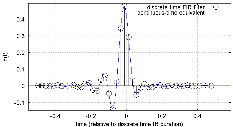

^{Fig. 1: Original discrete-time impulse response (black) and reconstructed continuous-time equivalent (blue)}

Applications:

• Can be used to illustrate the "meaning" behind unintuitive FIR coefficients, for example fractional delay banks in a polyphase filter.
• Shows the difficulty of "interpolating" by geometric means, i.e. polynomial, splines, etc, since the continuous-time waveform clearly depends on many (strictly speaking: all) supporting points.
• May provide a continuous-time impulse response for a (Farrow) resampler design, based on a discrete-time prototype.

Note:
The continuous-time equivalent impulse response of a discrete-time "finite impulse response" (FIR) filter is zero at all sampling instants beyond the duration of the discrete-time impulse response. However, it does not show the same finite duration as a whole.
The difference is subtle, but clearly visible for example on equiripple designs that exhibit a "discontinuous" last sample.

As is well-known, a linear-phase filter (without group delay dispersion) exhibits a symmetric impulse response. What is interesting here is that the continuous-time equivalent can be symmetric, even if the discrete-time impulse response appears asymmetrical (example: FIR with fractional-sample group delay).
_{Code tested on Octaveforge and Matlab}

% ************************************************************
% * Construct a continuous-time impulse response based on a discrete-time filter
% ************************************************************
close all; clear all;

% ************************************************************
% * example filter
% * f = [0 0.7 0.8 1]; a = [1 1 0 0];
% * b = remez(45, f, a);
% * h = b .';
% Illustrates rather clearly the difficulty of "interpolating" (in a geometric sense, 
% via polynomials, splines etc) between impulse response samples
% ************************************************************    
h = [2.64186706e-003 2.50796828e-003 -4.25450455e-003 4.82982358e-003 -2.51252769e-003 -2.52706568e-003 7.73569146e-003 -9.30398382e-003 4.65100223e-003 5.17152459e-003 -1.49409856e-002 1.76001904e-002 -8.65545521e-003 -9.78478603e-003 2.82103205e-002 -3.36173643e-002 1.68597129e-002 2.01914744e-002 -6.17486493e-002 8.13362871e-002 -4.80981494e-002 -8.05143565e-002 5.87677665e-001 5.87677665e-001 -8.05143565e-002 -4.80981494e-002 8.13362871e-002 -6.17486493e-002 2.01914744e-002 1.68597129e-002 -3.36173643e-002 2.82103205e-002 -9.78478603e-003 -8.65545521e-003 1.76001904e-002 -1.49409856e-002 5.17152459e-003 4.65100223e-003 -9.30398382e-003 7.73569146e-003 -2.52706568e-003 -2.51252769e-003 4.82982358e-003 -4.25450455e-003 2.50796828e-003 2.64186706e-003];

% ************************************************************
% zero-pad the impulse response of the FIR filter to 5x its original length
% (time domain)
% The filter remains functionally identical, since appending zero taps changes nothing
% ************************************************************
timePaddingFactor = 5;
n1 = timePaddingFactor * size(h, 2);
nh = size(h, 2);
nPad = n1 - nh;
nPad1 = floor(nPad / 2);
nPad2 = nPad - nPad1;
h = [zeros(1, nPad1), h, zeros(1, nPad2)];
hOrig = h;

% ************************************************************
% Determine equivalent Fourier series coefficients (frequency domain)
% assume that the impulse response is bandlimited (time-discrete signal by definition) 
% and periodic (period length see above, can be extended arbitrarily)
% ************************************************************
h = fft(h); % Fourier transform time domain to frequency domain

% ************************************************************
% Evaluate the Fourier series on an arbitrarily dense grid 
% this allows to resample the impulse response on an arbitrarily dense grid
% ************************************************************
% zero-pad Fourier transform
% ideal band-limited oversampling of the impulse response to n2 samples
n2 = 10 * n1;

h = [h(1:ceil(n1/2)), zeros(1, n2-n1), h(ceil(n1/2)+1:end)];
h = ifft(h); % back to time domain
% Note: One may write out the definition of ifft() and evaluate the exp(...) term at an 
% arbitrary time to acquire a true continuous-time equation.

% numerical inaccuracy in (i)fft causes some imaginary part ~1e-15
assert(max(abs(imag(h))) / max(abs(real(h))) < 1e-14);
h = real(h);

% scale to maintain amplitude level
h = h * n2 / n1;

% construct x-axis [0, 1[
xOrig = linspace(-timePaddingFactor/2, timePaddingFactor/2, size(hOrig, 2) + 1); xOrig = xOrig(1:end-1);
x = linspace(-timePaddingFactor/2, timePaddingFactor/2, size(h, 2) + 1); x = x(1:end-1);

% ************************************************************
% Plot 
% ************************************************************
% ... on a linear scale

% find points where original impulse response is defined (for illustration)
ixOrig = find(abs(hOrig) > 0);

figure(); grid on; hold on;
stem(xOrig(ixOrig), hOrig(ixOrig), 'k');
plot(x, h, 'b'); 
legend('discrete-time FIR filter', 'continuous-time equivalent');
title('equivalent discrete- and continuous-time filters');
xlabel('time (relative to discrete time IR duration)'); ylabel('h(t)');

% ... and again on a logarithmic scale
myEps = 1e-15;
figure(); grid on; hold on;
u = plot(xOrig(ixOrig), 20*log10(abs(hOrig(ixOrig)) + myEps), 'k+'); set(u, 'lineWidth', 3);
plot(x, 20*log10(abs(h) + myEps), 'b');
legend('discrete-time FIR filter', 'continuous-time equivalent');
title('equivalent discrete- and continuous-time filters');
xlabel('time (relative to discrete time IR duration)'); ylabel('|h(t)| / dB');