Remez (FIR design) weights from requirements

The Remez (Parks McClellan) method is commonly used for the design of FIR filters. It uses user-provided weighting factors that determine the filter accuracy in different bands. While they can be found by trial-and-error, this becomes cumbersome, especially in designs with many bands.

This code snippet shows how to calculate the weights, based on either a passband ripple or stopband attenuation requirement for each band.

Using the calculated weights, the filter will now either pass or fail all requirements simultaneously. What remains to be done is to find the required filter order, which is straightforward.

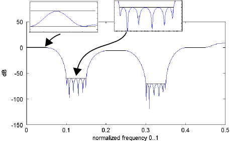
The plot shows the frequency response of the filter design example in the code snippet. It implements three passbands and two stopbands. One of the passbands was designed for -6 dB gain relative to the other two.
Zooming in reveals that the design requirements are met, without the need for manual "balancing" of accuracy between bands.

The explanation for the weighting factor equations can be found in the equiripple nature of a Remez-design with equal weights: The variation of |h(f)| on a linear scale is initially equal in passbands (where it appears around the nominal gain) and stopbands (centered at zero). The equations determine the ripple that is equivalent to the pass- / stopband-requirement, and scale the band's weight accordingly.

See also: A. Antoniou: IIR filters, tutorial, slide 49 and following.

^{Tested on OctaveForge and Matlab.}

% *********************************************
% Weighting factors for Remez equiripple FIR design
% M. Nentwig
% *********************************************
close all; clear all;

f = [0:9]/10; % normalized frequency 0..1

% a = nominal |H(f)| on a linear scale (sample amplitude)
% 1 1     : passband from frequency 0 to 0.1 
% 0 0     : stopband from frequency 0.2 to 0.3 
% 0.5 0.5 : passband with -6 dB (0.5 amplitude) from frequency 0.4 to 0.5 
% 0 0     : stopband from frequency 0.6 to 0.7
% 1 1     : passband from frequency 0.8 to 0.9
% other frequency ranges are "don't care" areas.
a = [1 1 0 0 0.5 0.5 0 0 1 1];

% *********************************************
% design specification for each band
% *********************************************
ripple1_dB = 0.3;
att2_dB = 60;
ripple3_dB = 0.2;
att4_dB = 70;
ripple5_dB = 0.1;

% *********************************************
% error for each band, on a linear scale
% *********************************************
% note: passband 3 has a nominal gain of 0.5 in 'a'.
% the allowed error of |H(f)| scales accordingly.
err1 = 1 - 10 ^ (-ripple1_dB / 20);
err2 = 10 ^ (-att2_dB / 20);
err3 = (1 - 10 ^ (-ripple3_dB / 20)) * 0.5; 
err4 = 10 ^ (-att4_dB / 20);
err5 = 1 - 10 ^ (-ripple5_dB / 20);

% the weight of each band is chosen as the inverse of the targeted error
% (stricter design target => higher weight).
% we could normalize each entry in w to (err1+err2+err3+err4+err5)
% but it would appear as common factor in all entries and therefore make no difference.
w = [1/err1 1/err2 1/err3 1/err4 1/err5];

% filter order
% this design problem is 'tweaked' so that the resulting filter is (quite) exactly on target
% for the given n, which can be changed only in steps of 1.
% Note that increasing order by 1 can make the filter worse due to even / odd 
% number of points (impulse response symmetry)
n = 52;

% *********************************************
% Run Remez / Parks McClellan filter design
% *********************************************
h = remez(n, f, a, w);
% force row vector (OctaveForge and Matlab's "remez" differ)
h = reshape(h, 1, prod(size(h))); 
% *********************************************
% Plot the results
% *********************************************
figure(1); hold on;

% zero-pad the impulse response to set frequency resolution
% of the FFT
h = [h, zeros(1, 1000)];

% frequency base
npts = size(h, 2);
fbase = (0:npts-1)/npts; 

plot(fbase, 20*log10(abs((fft(h)+1e-15))), 'b');
xlim([0, 0.5]);

% *********************************************
% sketch the requirements
% *********************************************
e = [1 1];
plot([f(1), f(2)]/2, e * ripple1_dB, 'k');
plot([f(1), f(2)]/2, e * -ripple1_dB, 'k');
plot([f(3), f(4)]/2, e * -att2_dB, 'k');
plot([f(5), f(6)]/2, e * ripple3_dB - 6.02, 'k');
plot([f(5), f(6)]/2, e * -ripple3_dB - 6.02, 'k');
plot([f(7), f(8)]/2, e * -att4_dB, 'k');
plot([f(9), f(10)]/2, e * ripple5_dB, 'k');
plot([f(9), f(10)]/2, e * -ripple5_dB, 'k');
xlabel('normalized frequency 0..1');
ylabel('dB');