


Yet Another FIR design algorithm
Designs real- or complex-valued FIR filters with linear or non-linear phase that match or equalize arbitrary frequency responses.
Update:
Download the latest version here (uses object-oriented syntax, split into multiple files, API cleanup).
Introduction
This code "snippet" will design FIR filters, simple ones and rather complex ones, too.
It may still succeed, where remez() runs into convergence problems. I haven't observed any such issues yet for realistic requirements.
The algorithm is also quite accessible (the Remez method is not for the faint-of-heart), making it useful for non-standard design problems that require customized programming.
Features:
- arbitrary number of passband- and stopbands with individual specifications, similar to remez().
- matches an arbitrary target frequency response, provided via simple lookup table
- equalizes (inverts) an arbitrary frequency response, for example to correct an analog filter
- linear or nonlinear phase (asymmetric impulse response, group delay distortion / equalization)
- symmetric or asymmetric spectrum (complex-valued impulse response)
- fractional-sample delay
- a comparison of the same (simple) design with an optimal equiripple filter from remez() shows a practically identical impulse response.
- can deliver (almost) equiripple designs
- alternatively, returns a least-mean-squares (LMS) optimal design
- or anything in-between
- makes coffee and walks the dog
- (maybe not)
Algorithm
I'll give here only a brief summary of the algorithm, since it's extensively documented in the code. I'm planning to write a blog entry on the topic later.
The algorithm
- generates a signal solverAtInput with passband energy only
- generates a signal solverAtOutput = solverAtInput
- applies the equalization target frequency response (if applicable) to solverAtInput
- applies the nominal frequency response (if applicable) to solverAtOutput
- generates an unwanted signal component that contains only stopband energy, and adds it to solverAtInput (this will force the LMS solver to implement stopband rejection)
- writes out the FIR equation solverAtOutput = sum of (tap weight) * (delayed solverAtInput)
- finds a LMS solution for the tap weights. Those are preliminary FIR coefficients.
- FIR-filters solverAtInput using the coefficients and compares with solverAtOutput
At this point, the FIR coefficients give the LMS-optimum FIR that maps solverAtInput to solverAtOutput.
Unfortunately, this "optimal" filter performs very well on frequencies where success comes easy, and neglects other frequencies, where improvement is more costly (see the "basicLMS" example for actual output).
As a result, the filter quality at transitions or band edges does not meet requirements, while the bulk of the frequency response exceeds them.
To address this issue and obtain equiripple results instead of LMS-optimal ones, the LMS solver is wrapped into an iteration loop as follows:
- create OriginalSolverAtInput and OriginalSolverAtOutput as described above
- initialize weighting factors
- Foreach iteration
- solverAtOutput = weight .* originalSolverAtOutput
- run the LMS solver
- If performance at frequency f needs to be improved
- then scale weighting factor for f by the required improvement
- if all targets are met, iterate a couple times more and then exit
- next iteration
Now there isn't too much need to understand any of the above, as long as the task at hand is only to design a FIR filter that meets given requirements. Simply run the program, edit as needed, and check that the output is meaningful (look out for excessive gain and wildly oscillating FIR taps with large absolute value).
Fortunately, verifying a FIR filter is much easier than designing one.
Equiripple or LMS-optimized?
For design requirements that are very close to what is achievable, the resulting design will be essentially equiripple (that is, all "bumps" in frequency response and error vector magnitude "touch" the requirement, or at least come close).
If the targets can be exceeded, the remaining freedom will be used (mostly) for LMS optimization. At first glance, it looks like sloppy work, when EVM and passband ripple start to "sag". But in many applications, a LMS optimization does make sense, beyond the point where requirements are met. See the "basic" and "basicLMS" demos for more details.
If equiripple is preferable, tighten the filter requirements iteratively, to the point where they are barely achievable. Results will approach equiripple, even though some bands may steadfastly refuse to deteriorate, if it doesn't gain an improvement elsewhere.
Optimal?
There is no guarantee that the iteration will converge to a global optimum. Small changes to the input of the LMS solver may result in an abrupt change in the placement of zeros, making the weighting factors meaningless.
Many other filter design methods aren't optimal, so this is not necessarily an issue for practical use.
If anybody can provide an example that shows non-optimality against a better design, I'd be very interested.
Detailed documentation
For now, all documentation is in the code. A number of complete, heavily documented design examples are included.
It may be also a good idea to look deeper into the functions, if needed. There are more comments and also a couple of plots that can be enabled.
Location of the core algorithm
Most of the code is "infrastructure" that provides a user interface to the second half of LMSFIR_stage3_run().
The essential part can be found in said function, enclosed within
for Iter
... pinv() ...
end
All signals are cyclic (infinite duration in the time domain, a finite Fourier series in the frequency domain).
Due to the cyclic nature, FFT and IFFT allow to go back and forth between time / frequency domain without any signal degradation other than numerical error. There is no need for any windowing, since the signal never starts or stops.
Further, causality is not an issue, time just wraps around.
Time domain variable names use the _td postfix, and _fd is used for frequency domain.
Bugs
While I've been using the core algorithm for quite a while now, this code snippet is a complete clean rewrite.
If you run into bugs, kindly let me know.
Matlab / OctaveForge
It is supposed to work on both.
Examples
All examples are included and can be called from the first few lines of the code snippet.
Simply uncomment one demo(...) line at a time and run.
In the plots below, the red trace gives the magnitude of the error vector, EVM (output signal minus input signal).
Ripple requirements are translated into EVM for plotting passband ripple and stopband rejection in one diagram.
demo("basic")
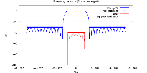
Fig.1: simple lowpass design example.
A filter to the same specifications can be designed with remez(). The filters are almost identical. Fig. 2 shows the impulse responses of both designs.
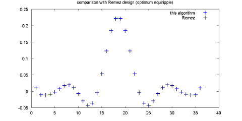
Fig. 2: Impulse response, compared to equivalent Remez design
demo("basicLMS")
Uses the same target settings as the "basic" demo, but does not iterate to achieve an equiripple solution.
The resulting design does not meet the requirements at pass- and stopband edge.
Given that the overall performance of the LMS design for a noise-like signal is about 5 dB better than the equiripple design in Fig. 1, this example illustrates that equiripple may come at a steep price, compared to LMS.
It also shows where the requirements are most "expensive": For example, raising either stop- or passband requirement at the edge slightly, or a small change in the band edge frequency, would significantly reduce the number of taps or improve performance elsewhere.
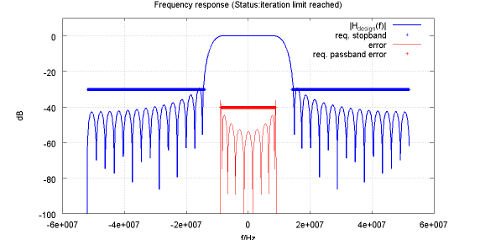
Fig 3: The same as the "basic" example, but LMS solution instead of equiripple
demo("stopband")
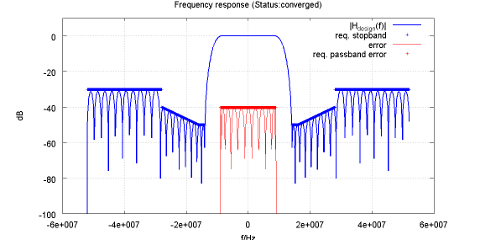
Fig. 4: Multiple stopbands
demo("multipassband")
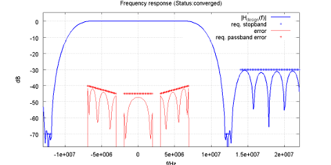
Fig. 5: Multiple passbands, with variable ripple / error.
demo("complex")
The frequency response in this example "runs away", because it is unconstrained around -40 MHz.
This problem can be solved by using a couple more taps and placing a "soft" stopband, for example 0 dB, in the "don't-care" regions.
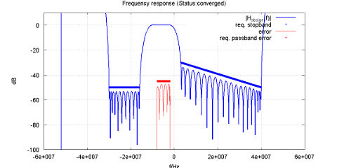
Fig. 6: Complex-valued FIR coefficients, asymmetric impulse response
demo("RRC")
Designs a filter with a root-raised cosine response for WCDMA cellular.
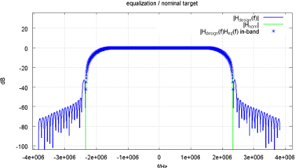
Fig. 7: Root-raised cosine design
demo("componentmodel")
In this example, the response of a 6th order Laplace-domain Chebyshev lowpass is modeled by a FIR filter.
Modeling IIR with FIR is a straightforward exercise, as long as the allowed number of taps is large. This is the case for wideband IIRs with short impulse response, and / or modest accuracy requirements: If possible, simply sample the impulse response, apply some windowing function and we're done (here is a discussion on textbook methods).
A general problem with IIRs is that the impulse response decays exponentially: Over time, it drops slower and slower. Reducing the truncated "tail" by using more taps may become impractical.
If so, a little bit of extra effort is required, as this example shows:
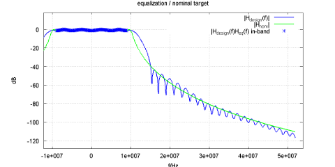
Fig. 8: Original IIR filter (green) and model (blue)
The model in this example carefully approximates the in-band response, for example to test a digital equalizer (Fig. 8 and 9). The model is phase-accurate within +/- 9 MHz.
The transition area around 12 MHz is left as "don't-care" region and therefore inaccurate.
The wide-band amplitude response is modeled using straight-line stopband requirements. The order of magnitude is more or less correct, but the model is not phase-accurate.
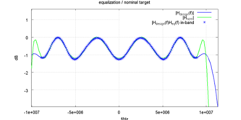
Fig. 9: IIR in-band model
demo("componentmodel2")
To add a twist to the previous example, let's assume the component model is meant for use in a radio receiver that attempts to demodulate a strong adjacent channel, even though it's on the edge of the analog filter.
A meaningful filter model needs to be phase-accurate in the frequency range in question. One solution is to add a second passband to the design script.
Note that since the gain ranges from -40 dB to -50 dB, the error vector requirement needs to be scaled down accordingly, to achieve a comparable signal quality as in the passband
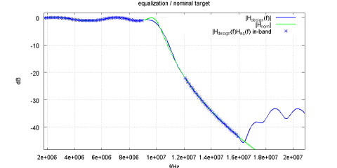
Fig. 10: FIR design to match a given frequency response in multiple passbands
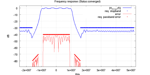
Fig. 11: EVM needs to be scaled relative to the passband gain to maintain signal quality
demo("equalize")
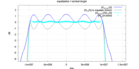
Fig. 12: Equalizing a given frequency response
Similar to the filter modeled in demo("component"), but now the filter is equalized instead of being used as nominal frequency response.
As the light blue trace shows, the frequency response that results from placing both filters in series is nearly flat. And, while not visible in the plots, also the phase is equalized. Since the equalizer is nonlinear phase, its impulse response is asymmetric and the group delay becomes a free parameter.
It is recommended to try different values and find the optimum. The performance is usually weakly periodic on a one-sample grid, because a "bad" value for the group delay effectively forces the equalizer to implement additional fractional delay that collapses to a unity sample at the optimum group delay.
comp.dsp
Here is a link to a discussion thread on comp.dsp.
Getting the code snippet
Download the latest version here (updated, split into multiple files). Unpack, cd into the folder and run YAFIR_demo_basic.
The code below can be also downloaded here / change log.
If using copy / paste, place it into a file named LMSFIR.m and run LMSFIR from the Matlab / OctaveForge command line.
% ********************************************
% least-mean-squares FIR design algorithm
% Markus Nentwig, 2010-2011
% release 2011/8/22
% ********************************************
function LMSFIR()
close all;
h1 = demo1('basic'); compareDemo1WithRemez(h1);
% h1 = demo1('basicLMS'); disp('demo: convergence failure is on purpose to show LMS solution');
% demo1('allpass');
% demo1('stopband');
% demo1('equalize');
% demo1('nominalResponse');
% demo1('multipassband');
% demo1('complex');
% demo1('rootRaisedCosineUpsampler');
% demo1('componentModel');
% demo1('componentModel2');
end
function h = demo1(nameOfDemo)
dpar = struct();
% parameters for a basic FIR lowpass filter design.
% kept in a struct(), so that individual examples
% can easily change them.
% sampling rate at the input of the filter
dpar.inRate_Hz = 104e6;
% number of physical FIR taps
% in a polyphase decimator, the number of internal
% coefficients will be fDecim * fStages
dpar.mStages = 36;
% end of passband. A single value will be internally
% expanded to [-9e6, 9e6].
% Asymmetric designs require
% the complexValued = true option.
% This 'default' passband can be omitted entirely, if passbands
% are declared individually later
dpar.req_passbandF_Hz = 9e6;
% defines the maximum allowed ripple in the passband.
dpar.req_passbandRipple_dB = 0.083;
% as alternative to ripple, the in-band error
% vector magnitude (EVM) can be limited
% dpar.req_passbandEVM_dB = -44;
% the passband specification may use multiple points
% dpar.req_passbandF_Hz = [-1, 5e6, 6e6, 9e6];
% dpar.req_passbandEVM_dB = [-44, -44, -34, -34];
% start of default stopband.
% as with the passband, the default stopband can be omitted,
% if individual bands are placed later.
dpar.req_stopbandF_Hz = 14e6;
dpar.req_stopbandMaxGain_dB = -30;
% dpar.req_stopbandF_Hz = [14e6, 34e6];
% dpar.req_stopbandGainMax_dB = [-30, -20];
% ********************************************
% create a filter design object "design"
% * access with LMSFIR_stage2 functions
% * evaluate with LMSFIR_stage3 function
% ********************************************
switch nameOfDemo
case 'basic'
% ********************************************
% simple filter using the parameters above
% ********************************************
design = LMSFIR_stage1_setup(dpar);
case 'basicLMS'
% ********************************************
% LMS design for comparison:
% Iterations are disabled
% ********************************************
dpar.nIter = 1;
% balance in-band / out-of-band performance as needed
dpar.inbandWeight_initValue = 5;
dpar.outOfBandWeight_initValue = 1;
design = LMSFIR_stage1_setup(dpar);
case 'allpass'
% ********************************************
% allpass design Offset the nominal delay by 1/3
% of a sample, compared to the "basic" example
% (compare the impulse responses)
% ********************************************
dpar.delayOffset = 1/3; % signal arrives now earlier
design = LMSFIR_stage1_setup(dpar);
case 'stopband'
% ********************************************
% Filter with added stopbands
% ********************************************
% the following features require more taps
dpar.mStages = 48;
% create filter design object
design = LMSFIR_stage1_setup(dpar);
% place a stopband from 14 to 16 MHz with -50 dB
design = LMSFIR_stage2_placeStopband(...
design, ...
'f_Hz', [14e6, 16e6], ...
'g_dB', [-50, -50]);
% place another stopband from 16 to 28 MHz with
% -50 dB, linearly relaxing to -40 dB
design = LMSFIR_stage2_placeStopband(...
design, ...
'f_Hz', [16e6, 28e6], ...
'g_dB', [-50, -40]);
case 'equalize'
% ********************************************
% Equalize the frequency response of another
% filter in the passband(s)
% ********************************************
% As an equalizer, this is rather inefficient with so much
% unused bandwidth. Should operate at the smallest possible BW instead.
dpar.mStages = 52;
[ffilter_Hz, H] = getExampleLaplaceDomainFilter();
% set the frequency points...
dpar.equalizeFreq_Hz = ffilter_Hz;
% ... and the filter response. The design routine will
% use linear interpolation, therefore provide a sufficiently
% dense grid.
% Equalizing an asymmetric response requires
% the complexValued=true option, leading to a complex-valued
% FIR filter.
% The equalization function needs to be normalized.
% Otherwise, pass- and stopband targets will be offset
% by the gain mismatch.
dpar.equalizeComplexGain = H;
% as alternative to the complex gain, a magnitude response
% can be given via an equalizeGain_dB argument.
% dpar.equalizeGain_dB = 20*log10(abs(H));
% an asymmetric (non-linear-phase) impulse response may
% require a group delay that is not centered in the
% FIR length.
dpar.delayOffset = 2;
design = LMSFIR_stage1_setup(dpar);
case 'componentModel'
% ********************************************
% Create a FIR filter that approximates the passband behavior of
% the analog filter accurately, and gives a similar stopband rejection
%
% The most straightforward way to model an infinite-impulse-response
% lowpass is to simply sample the impulse response. However, it needs to be
% cut to size (since the FIR filter has only finite length)
% => Chopping it off destroys the out-of-band performance (=rectangular window)
% => use a window function that trades off between passband accuracy and
% stopband rejection
% => or use the design example below.
% ********************************************
dpar.mStages = 52;
[ffilter_Hz, H] = getExampleLaplaceDomainFilter();
% set the frequency points...
dpar.nominalFreq_Hz = ffilter_Hz;
dpar.nominalComplexGain = H;
dpar.req_stopbandF_Hz = [15e6, 30e6, 55e6];
dpar.req_stopbandMaxGain_dB = [-38, -80, -115];
dpar.req_passbandF_Hz = 9e6;
% offset the impulse response, it is not centered
dpar.delayOffset = 18;
design = LMSFIR_stage1_setup(dpar);
case 'componentModel2'
% ********************************************
% an extension of "componentModel1"
% stopband rejection does not matter, but we need
% phase-accurate modeling on a region of the stopband edge
% ********************************************
dpar.mStages = 80; % this won't be cheap...
[ffilter_Hz, H] = getExampleLaplaceDomainFilter();
dpar.nominalFreq_Hz = ffilter_Hz;
dpar.nominalComplexGain = H;
dpar.req_stopbandF_Hz = [ 16e6, 100e6];
dpar.req_stopbandMaxGain_dB = [ -30, -30];
dpar.req_passbandF_Hz = 9e6;
% offset the impulse response, it is not centered
dpar.delayOffset = dpar.mStages / 2 - 8;
design = LMSFIR_stage1_setup(dpar);
% place a passband in the area on the slope that is to be modeled accurately
design = LMSFIR_stage2_placePassband(...
design, ...
'f_Hz', [12e6, 16e6], ...
'EVM_dB', [-40, -50] - 30); % nominal gain -40..-50 dB, -30 dBc EVM
case 'nominalResponse'
% ********************************************
% Design a filter to a given frequency response
% ********************************************
dpar.mStages = 50;
% the frequency response is approximated in any
% declared passband, but must be valid for any
% frequency to allow plotting.
dpar.nominalFreq_Hz = [0, 3e6, 9e6, 1e9];
dpar.nominalGain_dB = [0, 0, -6, -6];
% instead, nominalComplexGain can be used
% g = [0, 0, -3, -3];
% dpar.nominalComplexGain = 10 .^ (g/20);
design = LMSFIR_stage1_setup(dpar);
case 'multipassband'
% ********************************************
% Design a filter with three passbands
% ********************************************
dpar.mStages = 50;
dpar = rmfield(dpar, 'req_passbandF_Hz');
dpar = rmfield(dpar, 'req_passbandRipple_dB');
design = LMSFIR_stage1_setup(dpar);
design = LMSFIR_stage2_placePassband(...
design, ...
'f_Hz', [-2e6, 2e6], ...
'EVM_dB', -45);
design = LMSFIR_stage2_placePassband(...
design, ...
'f_Hz', [3e6, 7e6], ...
'EVM_dB', [-45, -40]);
design = LMSFIR_stage2_placeStopband(...
design, ...
'f_Hz', [11.8e6, 12.4e6], ...
'g_dB', -70);
case 'complex'
% ********************************************
% Design a complex-valued filter
% ********************************************
% this is also an example for what can go wrong:
% In the unconstrained section around -40 MHz, the
% frequency response is allowed to go berserk. Which
% it does.
% Solution: Place a "soft" stopband (for example at -5 dB)
% in the "don't-care" regions and add a couple of taps.
% remove passband from default parameters
dpar = rmfield(dpar, 'req_passbandF_Hz');
dpar = rmfield(dpar, 'req_passbandRipple_dB');
% remove stopband from default parameters
dpar = rmfield(dpar, 'req_stopbandF_Hz');
dpar = rmfield(dpar, 'req_stopbandMaxGain_dB');
dpar.complexValued = true;
design = LMSFIR_stage1_setup(dpar);
design = LMSFIR_stage2_placeStopband(...
design, ...
'f_Hz', [-30e6, -16e6], ...
'g_dB', -50);
design = LMSFIR_stage2_placePassband(...
design, ...
'f_Hz', [-8e6, -2e6], ...
'EVM_dB', -45);
design = LMSFIR_stage2_placeStopband(...
design, ...
'f_Hz', [3e6, 40e6], ...
'g_dB', [-30, -50]);
case 'rootRaisedCosineUpsampler'
% ********************************************
% root-raised cosine upsampling filter for WCDMA transmitter
% The input chip stream arrives at 3.84 Msps, using the
% full bandwidth.
% Before the filter, it is upsampled (zero insertion) to
% 7.68 Msps.
% The filter applies RRC-filtering with 1.22 rolloff.
% ********************************************
% calculate nominal RRC response for lookup table / linear
% interpolation
f_Hz = logspace(1, 8, 10000); f_Hz(1) = -1;
c = abs(f_Hz * 2 / 3.84e6);
c = (c-1)/(0.22); % -1..1 in the transition region
c=min(c, 1);
c=max(c, -1);
RRC_h = sqrt(1/2+cos(pi/2*(c+1))/2);
% ********************************************
% once the targets are achieved, use the remaining
% 'degrees of freedom' for least-squares optimization.
% The LMS solver will improve, where it is 'cheapest'
% The parameters are not a real-world design
% (0.5 percent EVM => -46 dB)
% ********************************************
ci = 0;
% ci = 10; % for comparison: force equiripple
dpar = struct(...
'inRate_Hz', 3.84e6, ...
'fInterp', 2, ...
'mStages', 45, ...
'req_passbandF_Hz', 3.84e6 * 1.22 / 2, ...
'req_passbandEVM_dB', -46, ...
'req_stopbandF_Hz', 2.46e6, ...
'req_stopbandMaxGain_dB', -50, ...
'nominalFreq_Hz', f_Hz, ...
'nominalGain_dB', 20*log10(RRC_h + 1e-19), ...
'convergedIterations', ci);
design = LMSFIR_stage1_setup(dpar);
[h, status] = LMSFIR_stage3_run(design);
% save('hRRC_upsampler.txt', 'h', '-ascii');
disp(status);
otherwise
assert(false);
end % switch nameOfDemo
% ********************************************
% Design the filter
% ********************************************
% h is the impulse response (FIR tap coefficients).
[h, status] = LMSFIR_stage3_run(design);
disp(status);
end
function compareDemo1WithRemez(hLMS)
% identical target settings to demo1 "basic".
% note, the demo uses targets that are exactly "on the edge"
% what the algorithm can achieve. This results in an equiripple-
% design that can be compared with remez().
% If the targets are too loosely set, pass- and stopband quality
% start to "sag" in the band middle (LMS solution => lowest overall
% error, the optimizer improves where it's "cheapest").
r_Hz = 104e6;
m = 35; % definition differs by 1
f = [0 9e6 14e6 r_Hz/2] / (r_Hz/2);
a = [1 1 0 0];
ripple_dB = 0.1;
att_dB = 30;
err1 = 1 - 10 ^ (-ripple_dB / 20);
err2 = 10 ^ (-att_dB / 20);
w = [1/err1 1/err2];
% get remez design impulse response
hRemez = remez(m, f, a, w);
figure(); hold on;
handle = plot(hLMS, 'b+'); set(handle, 'lineWidth', 3);
plot(hRemez, 'k+'); set(handle, 'lineWidth', 2);
legend('this algorithm', 'Remez');
title('comparison with Remez design (optimum equiripple)');
end
% Gets the frequency response of an "analog" (Laplace-domain) filter.
% => Chebyshev response
% => 6th order
% => 1.2 dB ripple
% => cutoff frequency at 10 MHz
% returns
% f_Hz: list of frequencies
% H: complex-valued H(f_Hz)
function [f_Hz, H] = getExampleLaplaceDomainFilter()
[IIR_b, IIR_a] = cheby1(6, 1.2, 1, 's');
% evaluate it on a wide enough frequency range
f_Hz = logspace(1, 10, 1000); f_Hz(1) = -1;
% Laplace domain operator for normalized frequency
fCutoff_Hz = 10e6;
s = 1i * f_Hz / fCutoff_Hz;
% polynomial in s
H_num = polyval(IIR_b, s);
H_denom = polyval(IIR_a, s);
H = H_num ./ H_denom;
end
% === LMSFIR_xyz "API" functions ===
% ********************************************
% LMSFIR_stagex_... functions to interact with design 'object'
% to be executed in 'stage'-order
% ********************************************
function d = LMSFIR_stage1_setup(varargin)
p = varargin2struct(varargin);
d = struct();
% number of frequency points. Increase to improve accuracy.
% Frequencies are quantized to +/- rate / (2 * nSamples)
d.nSamples = 1024;
% default polyphase interpolation: none
d.fInterp = 1;
% default polyphase decimation: none
d.fDecim = 1;
% max. number of iterations
d.nIter = 100;
% for pure LMS solution, set nIter to 1 and change the weights below as needed
d.inbandWeight_initValue = 1;
d.outOfBandWeight_initValue = 1;
% abort when the iteration weights grow too large.
% This happens when targets are impossible.
% The result may still be meaningful, though.
d.abortWeight = 1e12;
% keep iterating, if the targets are reached.
% Once the "equi"-ripple iteration has brought all peaks to an acceptable level,
% the LMS solver will use the remaining "degrees of freedom" for a LMS optimization.
% The solver improves "where it is easy / cheap". This results in sloped
% stopbands and "drooping" EVM in passbands.
% Often, LMS is the best choice => set converged iterations to 0.
d.convergedIterations = 10;
% for a complex-valued filter, use "true".
% With a real-valued design, user input is only evaluated for positive frequencies!
d.complexValued = false;
% by default, the basis waveforms given to the optimizer are
% within a delay range of +/- half the FIR length.
% For nonlinear phase types (equalization / nominal frequency
% response), this may be suboptimal.
% Meaningful values shouldn't exceed +/- half the number of
% coefficients in the impulse response.
d.delayOffset = 0;
% copy parameters
fn = fieldnames(p);
for ix = 1:size(fn, 1)
key = fn{ix};
d.(key) = p.(key);
end
% frequency base over FFT range
fb = 0:(d.nSamples - 1);
fb = fb + floor(d.nSamples / 2);
fb = mod(fb, d.nSamples);
fb = fb - floor(d.nSamples / 2);
fb = fb / d.nSamples; % now [0..0.5[, [-0.5..0[
fb = fb * d.inRate_Hz * d.fInterp;
d.fb = fb;
% in real-valued mode, negative frequencies are treated as
% positive, when 'user input' is evaluated
if d.complexValued
d.fbUser = fb;
else
d.fbUser = abs(fb);
end
% ********************************************
% target settings. Those will be modified by
% LMSFIR_stage2_xyz()
% ********************************************
% initial value of NaN indicates: all entries are unset
d.errorSpecBinVal_inband_dB = zeros(size(d.fb)) + NaN;
d.errorSpecBinVal_outOfBand_dB = zeros(size(d.fb)) + NaN;
% ********************************************
% process req_passband requirement
% needs to be done at stage 1, because it is
% used for 'gating' with the tightenExisting /
% relaxExisting options
% ********************************************
if isfield(d, 'req_passbandF_Hz')
par = struct('onOverlap', 'error');
if isfield(d, 'req_passbandRipple_dB')
par.ripple_dB = d.req_passbandRipple_dB;
end
if isfield(d, 'req_passbandEVM_dB')
par.EVM_dB = d.req_passbandEVM_dB;
end
par.f_Hz = d.req_passbandF_Hz;
d = LMSFIR_stage2_placePassband(d, par);
end % if req_passbandF_Hz
% ********************************************
% process req_stopband requirement
% needs to be done at stage 1, because it is
% used for 'gating' with the tightenExisting /
% relaxExisting options
% ********************************************
if isfield(d, 'req_stopbandF_Hz')
f_Hz = d.req_stopbandF_Hz;
g_dB = d.req_stopbandMaxGain_dB;
% extend to infinity
if isscalar(f_Hz)
f_Hz = [f_Hz 9e19];
g_dB = [g_dB g_dB(end)];
end
d = placeBand...
(d, ...
'f_Hz', f_Hz, 'g_dB', g_dB, ...
'type', 'stopband', ...
'onOverlap', 'tighten');
end
% ********************************************
% plot management
% ********************************************
d.nextPlotIx = 700;
end
function d = LMSFIR_stage2_placeStopband(d, varargin)
p = varargin2struct(varargin);
% shorthand notation g_dB = -30; f_Hz = 9e6;
% extend fixed passband to positive infinity
if isscalar(p.f_Hz)
assert(p.f_Hz > 0);
p.f_Hz = [p.f_Hz 9e99];
end
if isscalar(p.g_dB)
p.g_dB = ones(size(p.f_Hz)) * p.g_dB;
end
% default action is to use the stricter requirement
if ~isfield(p, 'onOverlap')
p.onOverlap = 'tighten';
end
d = placeBand(d, 'type', 'stopband', p);
end
function d = LMSFIR_stage2_placePassband(d, varargin)
p = varargin2struct(varargin);
% default action is to use the stricter requirement
if ~isfield(p, 'onOverlap')
p.onOverlap = 'tighten';
end
% translate ripple spec to error
if isfield(p, 'ripple_dB')
assert(p.ripple_dB > 0);
eSamplescale = 10 ^ (p.ripple_dB / 20) - 1;
EVM_dB = 20*log10(eSamplescale);
end
if isfield(p, 'EVM_dB')
EVM_dB = p.EVM_dB;
end
% convert scalar to two-element vector
if isscalar(EVM_dB)
EVM_dB = [EVM_dB EVM_dB];
end
% *** handle f_Hz ***
f_Hz = p.f_Hz;
% extend to 0 Hz
if isscalar(f_Hz)
f_Hz = [0 f_Hz];
end
% *** create the passband ***
d = placeBand(d, ...
'type', 'passband', ...
'f_Hz', f_Hz, ...
'g_dB', EVM_dB, ...
'onOverlap', p.onOverlap);
end
% ********************************************
% the filter design algorithm
% h: impulse response
% status: converged or not
% note that even if convergence was not reached,
% the resulting impulse response is "the best we
% can do" and often meaningful.
% ********************************************
function [h, status] = LMSFIR_stage3_run(d)
1;
% mTaps is number of physical FIR stages
% m is number of polyphase coefficients
d.m = d.mStages * d.fInterp;
% masks flagging pass-/stopband frequencies
mask_inband = NaN_to_0_else_1(d.errorSpecBinVal_inband_dB);
mask_outOfBand = NaN_to_0_else_1(d.errorSpecBinVal_outOfBand_dB);
% sanity check... (orthogonality of wanted and unwanted component)
assert(sum(mask_inband) > 0, 'passband is empty');
assert(sum(mask_inband .* mask_outOfBand) == 0, ...
'passband and stopband overlap');
% ********************************************
% start with flat passband signals at input and output of filter
% those will become the input to the LMS solver.
% ********************************************
sigSolverAtInput_fd = mask_inband;
sigSolverAtOutput_fd = sigSolverAtInput_fd;
% ********************************************
% for even-sized FFT length, there is one bin at the
% Nyquist limit that gives a [-1, 1, -1, 1] time domain
% waveform. It has no counterpart with opposite frequency
% sign and is therefore problematic (time domain component
% cannot be delayed).
% Don't assign any input power here.
% ********************************************
if mod(d.nSamples, 2) == 0
ixNyquistBin = floor(d.nSamples/2) + 1;
sigSolverAtInput_fd(ixNyquistBin) = 0;
sigSolverAtOutput_fd(ixNyquistBin) = 0;
end
if isfield(d, 'equalizeFreq_Hz')
% ********************************************
% Filter equalizes a given passband frequency response
% ********************************************
if isfield(d, 'equalizeGain_dB')
cgain = 10 .^ (equalizeGain_dB / 20);
else
cgain = d.equalizeComplexGain;
end
d.Heq = evaluateFilter(d.fb, d.equalizeFreq_Hz, cgain, d.complexValued);
assert(isempty(find(isnan(d.Heq), 1)), ...
['equalizer frequency response interpolation failed. ' ...
'Please provide full range data for plotting, even if it does not ', ...
'affect the design']);
% ********************************************
% apply frequency response to input signal.
% The LMS solver will invert this response
% ********************************************
sigSolverAtInput_fd = sigSolverAtInput_fd .* d.Heq;
end
if isfield(d, 'nominalFreq_Hz')
% ********************************************
% (equalized) filter matches a given passband frequency response
% ********************************************
if isfield(d, 'nominalGain_dB')
cgain = 10 .^ (d.nominalGain_dB / 20);
else
cgain = d.nominalComplexGain;
end
d.Hnom = evaluateFilter(d.fb, d.nominalFreq_Hz, cgain, d.complexValued);
assert(isempty(find(isnan(d.Hnom), 1)), ...
['nominal frequency response interpolation failed. ' ...
'Please provide full range data for plotting, even if it does not ', ...
'affect the design']);
% ********************************************
% apply frequency response to output signal.
% The LMS solver will adapt this response
% ********************************************
sigSolverAtOutput_fd = sigSolverAtOutput_fd .* d.Hnom;
end
% ********************************************
% compensate constant group delay from equalizer and nominal
% frequency response. This isn't optimal, but it is usually
% a good starting point (use delayOffset parameter)
% ********************************************
[coeff, ref_shiftedAndScaled, deltaN] = fitSignal_FFT(...
ifft(sigSolverAtInput_fd), ifft(sigSolverAtOutput_fd));
% the above function also scales for best fit. This is not desired here, instead
% let the LMS solver match the gain. Simply scale it back:
ref_shifted = ref_shiftedAndScaled / coeff;
sigSolverAtOutput_fd = fft(ref_shifted);
if false
% ********************************************
% plot time domain waveforms (debug)
% ********************************************
figure(76); hold on;
plot(fftshift(abs(ifft(sigSolverAtOutput_fd))), 'k');
plot(fftshift(abs(ifft(sigSolverAtInput_fd))), 'b');
title('time domain signals');
legend('reference (shifted)', 'input signal');
end
% ********************************************
% main loop of the design algorithm
% => initialize weights
% => loop
% => design optimum LMS filter that transforms weighted input
% into weighted output
% => adapt weights
% => iterate
% ********************************************
% at this stage, the input to the algorithm is as follows:
% => errorSpec for in-band and out-of-band frequencies
% (masks are redundant, can be derived from above)
% => LMS_in_fd and
% => LMS_out_fd: Signals that are given to the LMS solver.
% Its task is: "design a FIR filter that transforms LMS_in_fd into LMS_out_fd".
% initialize weights
outOfBandWeight = mask_outOfBand * d.outOfBandWeight_initValue;
inbandWeight = mask_inband * d.inbandWeight_initValue;
status = '? invalid ?';
hConv = [];
remConvIter = d.convergedIterations;
for iter=1:d.nIter
% inband weight is applied equally to both sides to shape the error
% out-of-band weight is applied to the unwanted signal
LMS_in_fd = sigSolverAtInput_fd .* inbandWeight...
+ mask_outOfBand .* outOfBandWeight;
LMS_out_fd = sigSolverAtOutput_fd .* inbandWeight;
% ********************************************
% cyclic time domain waveforms from complex spectrum
% ********************************************
LMS_in_td = ifft(LMS_in_fd);
LMS_out_td = ifft(LMS_out_fd);
% ********************************************
% construct FIR basis (output per coeffient)
% time domain waveforms, shifted according to each FIR tap
% ********************************************
basis = zeros(d.m, d.nSamples);
% introduce group delay target
ix1 = -d.m/2+0.5 + d.delayOffset;
ix2 = ix1 + d.m - 1;
rowIx = 1;
for ix = ix1:ix2 % index 1 appears at ix1
basis(rowIx, :) = FFT_delay(LMS_in_td, ix);
rowIx = rowIx + 1;
end
if d.complexValued
rightHandSide_td = LMS_out_td;
else
% use real part only
basis = [real(basis)];
rightHandSide_td = [real(LMS_out_td)];
pRp = real(rightHandSide_td) * real(rightHandSide_td)' + eps;
pIp = imag(rightHandSide_td) * imag(rightHandSide_td)';
assert(pIp / pRp < 1e-16, ...
['got an imaginary part where there should be none. ', ...
'uncomment the following lines, if needed']);
% if designing a real-valued equalizer for a complex-valued frequency response,
% use the following to solve LMS over the average:
% basis = [real(basis) imag(basis)];
% rightHandSide_td = [real(LMS_out_td), imag(LMS_out_td)];
end
% ********************************************
% LMS solver
% find a set of coefficients that scale the
% waveforms in "basis", so that their sum matches
% "rightHandSide_td" LMS-optimally
% ********************************************
pbasis = pinv(basis .');
h = transpose(pbasis * rightHandSide_td .');
% pad impulse response to n
irIter = [h, zeros(1, d.nSamples-d.m)];
% undo the nominal group delay
irIter = FFT_delay(irIter, ix1);
HIter = fft(irIter);
% ********************************************
% filter test signal
% ********************************************
eq_fd = sigSolverAtInput_fd .* HIter;
% ********************************************
% subtract actual output from targeted output
% results in error spectrum
% ********************************************
err_fd = sigSolverAtOutput_fd - eq_fd;
err_fd = err_fd .* mask_inband; % only in-band matters
EVM_dB = 20*log10(abs(err_fd)+1e-15);
% ********************************************
% out-of-band leakage
% ********************************************
leakage_dB = 20*log10(abs(HIter .* mask_outOfBand + 1e-15));
% ********************************************
% compare achieved and targeted performance
% ********************************************
deltaLeakage_dB = leakage_dB - d.errorSpecBinVal_outOfBand_dB;
deltaEVM_dB = EVM_dB - d.errorSpecBinVal_inband_dB;
% ********************************************
% find bins where performance should be improved
% or relaxed
% ********************************************
ixImprLeakage = find(deltaLeakage_dB > 0);
ixImprEVM = find(deltaEVM_dB > 0);
ixRelLeakage = find(deltaLeakage_dB < -3);
ixRelEVM = find(deltaEVM_dB < -3);
status = 'iteration limit reached';
if isempty(ixImprLeakage) && isempty(ixImprEVM)
% both targets met. Convergence!
if remConvIter > 0
remConvIter = remConvIter - 1;
status = 'converged once, now trying to improve';
hConv = h;
else
status = 'converged';
break;
end
end
% ********************************************
% improve / relax in-band and out-of-band
% ********************************************
if ~isempty(ixImprLeakage)
% tighten out-of-band
outOfBandWeight(ixImprLeakage) = outOfBandWeight(ixImprLeakage)...
.* 10 .^ ((deltaLeakage_dB(ixImprLeakage) + 0.1) / 20);
end
if ~isempty(ixRelLeakage)
% relax out-of-band
outOfBandWeight(ixRelLeakage) = outOfBandWeight(ixRelLeakage)...
.* 10 .^ (deltaLeakage_dB(ixRelLeakage) / 3 / 20);
end
if ~isempty(ixImprEVM)
% tighten in-band
inbandWeight(ixImprEVM) = inbandWeight(ixImprEVM)...
.* 10 .^ ((deltaEVM_dB(ixImprEVM) + 0.01) / 20);
end
if ~isempty(ixRelEVM)
% relax in-band
inbandWeight(ixRelEVM) = inbandWeight(ixRelEVM)...
.* 10 .^ (deltaEVM_dB(ixRelEVM) / 2 / 20);
end
if max([inbandWeight, outOfBandWeight] > d.abortWeight)
status = 'weight vector is diverging';
break;
end
end % for iter
% ********************************************
% recover from convergence failure after convergence
% during improvement phase
% ********************************************
if ~strcmp(status, 'converged')
if ~isempty(hConv)
h = hConv;
status = 'converged';
end
end
if true
% ********************************************
% plot impulse response
% ********************************************
if d.complexValued
figure(); hold on;
stem(real(h), 'k');
stem(imag(h), 'b');
legend('real(h)', 'imag(h)');
else
figure(); hold on;
stem(h);
legend('h');
end
title('impulse response');
end
% ********************************************
% plot frequency response
% ********************************************
inbandBins = find(mask_inband);
outOfBandBins = find(mask_outOfBand);
d=doPlotStart(d, ['Frequency response (Status:', status, ')']);
d=doPlotH(d, HIter, 'b', '|H_{design}(f)|', 2);
handle = plot(d.fb(outOfBandBins), d.errorSpecBinVal_outOfBand_dB(outOfBandBins), 'b+');
set(handle, 'markersize', 2);
d=addLegend(d, 'req. stopband');
d = doPlot_dB(d, EVM_dB, 'r', 'error');
handle = plot(d.fb(inbandBins), d.errorSpecBinVal_inband_dB(inbandBins), 'r+');
set(handle, 'markersize', 2);
d=addLegend(d, 'req. passband error');
d=doPlotEnd(d);
ylim([-100, 10]);
if false
% ********************************************
% plot constraint signal and weights
% ********************************************
figure(31); grid on; hold on;
handle = plot(fftshift(d.fb), fftshift(20*log10(mask_outOfBand)));
set(handle, 'lineWidth', 3);
x = d.fb; y = 20*log10(inbandWeight / max(inbandWeight));
handle = plot(x(inbandBins), y(inbandBins), 'k+'); set(handle, 'lineWidth', 3);
x = d.fb;
y = 20*log10(outOfBandWeight / max(outOfBandWeight));
handle = plot(x(outOfBandBins), y(outOfBandBins), 'b+'); set(handle, 'lineWidth', 3);
xlabel('f/Hz'); ylabel('dB');
ylim([-80, 40]);
legend('constraint signal', 'in-band weight', 'out-of-band weight');
title('weighting factor (normalized to 0 dB)');
end
hasEq = isfield(d, 'Heq');
hasNom = isfield(d, 'Hnom');
if hasEq || hasNom
% ********************************************
% plot equalization / nominal target
% ********************************************
d=doPlotStart(d, 'equalization / nominal target');
d=doPlotH(d, HIter, 'b', '|H_{design}(f)|', 2);
if hasEq
d=doPlotH(d, d.Heq, 'k', '|H_{eq}(f)| to equalize (invert)');
eqR = HIter .* d.Heq;
d=doPlotH(d, eqR, 'c', '|H_{design}(f)H_{eq}(f)|', 2);
handle = plot(d.fb(inbandBins), ...
20*log10(abs(eqR(inbandBins)) + 1e-15), 'c*');
set(handle, 'markersize', 3);
d=addLegend(d, '|H_{eq}(in-band)');
end
if hasNom
d = doPlotH(d, d.Hnom, 'g', '|H_{nom}|', 2);
handle = plot(d.fb(inbandBins), ...
20*log10(abs(HIter(inbandBins)) + 1e-15), 'b*');
set(handle, 'markersize', 3);
d=addLegend(d, '|H_{design}(f)H_{eq}(f) in-band');
end
d=doPlotEnd(d);
% set y-range
ymax = 20*log10(max(abs(HIter)));
ylim([-50, ymax+3]);
end
end
% === LMSFIR helper functions ===
% evaluates frequency response f_dB; g_Hz at fb
% the return value will contain NaN for out-of-range entries
% in fb
function binVal = buildBinVal(varargin)
p = varargin2struct(varargin);
f_Hz = p.f_Hz;
g_dB = p.g_dB;
% shorthand notation f = [f1, f2]; g = -30;
if isscalar(g_dB)
g_dB = ones(size(f_Hz)) * g_dB;
end
% tolerate sloppy two-argument definition
if size(f_Hz, 2) == 2 && f_Hz(1) > f_Hz(2)
f_Hz = fliplr(f_Hz);
g_dB = fliplr(g_dB);
end
binVal = interp1(f_Hz, g_dB, p.fbUser, 'linear');
end
function d = placeBand(d, varargin)
p = varargin2struct(varargin);
% create requirements vector
binVal = buildBinVal('f_Hz', p.f_Hz, ...
'g_dB', p.g_dB, ...
'fbUser', d.fbUser);
% look up requirements vector from design object
switch p.type
case 'passband'
fn = 'errorSpecBinVal_inband_dB';
case 'stopband'
fn = 'errorSpecBinVal_outOfBand_dB';
otherwise
assert(false);
end
designObject_binVal = d.(fn);
% check overlap
if strcmp(p.onOverlap, 'error')
m1 = NaN_to_0_else_1(designObject_binVal);
m2 = NaN_to_0_else_1(binVal);
assert(isempty(find(m1 .* m2, 1)), ...
['newly declared band overlaps existing band, '...
'which was explicitly forbidden by onOverlap=error']);
p.onOverlap = 'tighten'; % there won't be overlap,
% merging is dummy operation
end
% merging rules
switch p.onOverlap
case 'tighten'
logicOp = 'or';
valueOp = 'min';
case 'relax'
logicOp = 'or';
valueOp = 'max';
case 'tightenExisting'
logicOp = 'and';
valueOp = 'min';
case 'relaxExisting'
logicOp = 'and';
valueOp = 'max';
otherwise
assert(false);
end
% merge requirements tables
binValMerged = mergeBinVal(...
'binVal1', designObject_binVal, ...
'binVal2', binVal, ...
'logicalOperator', logicOp, ...
'valueOperator', valueOp);
% assign new requirements table
d.(fn) = binValMerged;
end
function r = NaN_to_0_else_1(vec)
r = zeros(size(vec));
% logical indexing, instead of r(find(~isnan(vec))) = 1;
r(~isnan(vec)) = 1;
end
function binVal = mergeBinVal(varargin)
p = varargin2struct(varargin);
% region where first argument is defined
mask1 = NaN_to_0_else_1(p.binVal1);
% region where second argument is defined
mask2 = NaN_to_0_else_1(p.binVal2);
% region where result will be defined
switch(p.logicalOperator)
case 'or'
mask = mask1 + mask2;
case 'and'
mask = mask1 .* mask2;
otherwise
assert(false);
end
ix = find(mask);
% merge into result
binVal = zeros(size(p.binVal1)) + NaN;
switch(p.valueOperator)
case 'min'
% note: The function min/max ignore NaNs (see "min" man
% page in Matlab)
% if one entry is NaN, the other entry will be returned
binVal(ix) = min(p.binVal1(ix), p.binVal2(ix));
case 'max'
binVal(ix) = max(p.binVal1(ix), p.binVal2(ix));
otherwise
assert(false);
end
end
% evaluates [f / gain] filter specification on the frequency grid
function H = evaluateFilter(f_eval, modelF, modelH, complexValued)
oneSided = false;
if ~complexValued
oneSided = true;
else
if min(modelF) > min(f_eval)
disp(['Warning: Filter model does not contain (enough) negative frequencies. ', ...
'assuming symmetric H(f) / real-valued h(t)']);
oneSided = true;
end
end
if oneSided
f_evalOrig = f_eval;
f_eval = abs(f_eval);
end
H = interp1(modelF, modelH, f_eval, 'linear');
if oneSided
% enforce symmetry (=> real-valued impulse response)
logicalIndex = (f_evalOrig < 0);
H(logicalIndex) = conj(H(logicalIndex));
end
end
function [d, handle] = doPlotH(d, H, spec, legEntry, linewidth)
handle = plot(fftshift(d.fb), fftshift(20*log10(abs(H)+1e-15)), spec);
d = addLegend(d, legEntry);
if exist('linewidth', 'var')
set(handle, 'lineWidth', linewidth);
end
end
function [d, handle] = doPlot_dB(d, H, spec, legEntry, linewidth)
handle = plot(fftshift(d.fb), fftshift(H), spec);
d.legList{size(d.legList, 2) + 1} = legEntry;
if exist('linewidth', 'var')
set(handle, 'lineWidth', linewidth);
end
end
function d = doPlotStart(d, plotTitle)
figure(d.nextPlotIx);
title(plotTitle);
grid on; hold on;
d.nextPlotIx = d.nextPlotIx + 1;
d.legList = {};
end
function d = doPlotEnd(d)
legend(d.legList);
xlabel('f/Hz');
ylabel('dB');
end
function d = addLegend(d, legEntry)
d.legList{size(d.legList, 2) + 1} = legEntry;
end
% === general-purpose library functions ===
% handling of function arguments
% someFun('one', 1, 'two', 2, 'three', 3) => struct('one', 1, 'two', 2, 'three', 3)
% a struct() may appear in place of a key ('one') and gets merged into the output.
function r = varargin2struct(arg)
assert(iscell(arg));
switch(size(arg, 2))
case 0 % varargin was empty
r=struct();
case 1 % single argument, wrapped by varargin into a cell list
r=arg{1}; % unwrap
assert(isstruct(r));
otherwise
r=struct();
% iterate through cell elements
ix=1;
ixMax=size(arg, 2);
while ix <= ixMax
e=arg{ix};
if ischar(e)
% string => key/value. The next field is a value
ix = ix + 1;
v = arg{ix};
r.(e) = v;
elseif isstruct(e)
names = fieldnames(e);
assert(size(names, 2)==1); % column
for ix2 = 1:size(names, 1)
k = names{ix2};
v = e.(k);
r.(k) = v;
end
else
disp('invalid token in vararg handling. Expecting key or struct. Got:');
disp(e);
assert(false)
end
ix=ix+1;
end % while
end % switch
end
function sig = FFT_delay(sig, nDelay)
sig = fft(sig); % to frequency domain
nSigSamples = size(sig, 2);
binFreq=(mod(((0:nSigSamples-1)+floor(nSigSamples/2)), nSigSamples)-floor(nSigSamples/2));
phase = -2*pi*nDelay / nSigSamples .* binFreq;
rot = exp(1i*phase);
if mod(nSigSamples, 2)==0
% even length - bin at Nyquist limit
rot(nSigSamples/2+1)=cos(phase(nSigSamples/2+1));
end
sig = sig .* rot;
sig = ifft(sig); % to time domain
end
% *******************************************************
% delay-matching between two signals (complex/real-valued)
%
% * matches the continuous-time equivalent waveforms
% of the signal vectors (reconstruction at Nyquist limit =>
% ideal lowpass filter)
% * Signals are considered cyclic. Use arbitrary-length
% zero-padding to turn a one-shot signal into a cyclic one.
%
% * output:
% => coeff: complex scaling factor that scales 'ref' into 'signal'
% => delay 'deltaN' in units of samples (subsample resolution)
% apply both to minimize the least-square residual
% => 'shiftedRef': a shifted and scaled version of 'ref' that
% matches 'signal'
% => (signal - shiftedRef) gives the residual (vector error)
%
% Example application
% - with a full-duplex soundcard, transmit an arbitrary cyclic test signal 'ref'
% - record 'signal' at the same time
% - extract one arbitrary cycle
% - run fitSignal
% - deltaN gives the delay between both with subsample precision
% - 'shiftedRef' is the reference signal fractionally resampled
% and scaled to optimally match 'signal'
% - to resample 'signal' instead, exchange the input arguments
% *******************************************************
function [coeff, shiftedRef, deltaN] = fitSignal_FFT(signal, ref)
n=length(signal);
% xyz_FD: Frequency Domain
% xyz_TD: Time Domain
% all references to 'time' and 'frequency' are for illustration only
forceReal = isreal(signal) && isreal(ref);
% *******************************************************
% Calculate the frequency that corresponds to each FFT bin
% [-0.5..0.5[
% *******************************************************
binFreq=(mod(((0:n-1)+floor(n/2)), n)-floor(n/2))/n;
% *******************************************************
% Delay calculation starts:
% Convert to frequency domain...
% *******************************************************
sig_FD = fft(signal);
ref_FD = fft(ref, n);
% *******************************************************
% ... calculate crosscorrelation between
% signal and reference...
% *******************************************************
u=sig_FD .* conj(ref_FD);
if mod(n, 2) == 0
% for an even sized FFT the center bin represents a signal
% [-1 1 -1 1 ...] (subject to interpretation). It cannot be delayed.
% The frequency component is therefore excluded from the calculation.
u(length(u)/2+1)=0;
end
Xcor=abs(ifft(u));
% figure(); plot(abs(Xcor));
% *******************************************************
% Each bin in Xcor corresponds to a given delay in samples.
% The bin with the highest absolute value corresponds to
% the delay where maximum correlation occurs.
% *******************************************************
integerDelay = find(Xcor==max(Xcor));
% (1): in case there are several bitwise identical peaks, use the first one
% Minus one: Delay 0 appears in bin 1
integerDelay=integerDelay(1)-1;
% Fourier transform of a pulse shifted by one sample
rotN = exp(2i*pi*integerDelay .* binFreq);
uDelayPhase = -2*pi*binFreq;
% *******************************************************
% Since the signal was multiplied with the conjugate of the
% reference, the phase is rotated back to 0 degrees in case
% of no delay. Delay appears as linear increase in phase, but
% it has discontinuities.
% Use the known phase (with +/- 1/2 sample accuracy) to
% rotate back the phase. This removes the discontinuities.
% *******************************************************
% figure(); plot(angle(u)); title('phase before rotation');
u=u .* rotN;
% figure(); plot(angle(u)); title('phase after rotation');
% *******************************************************
% Obtain the delay using linear least mean squares fit
% The phase is weighted according to the amplitude.
% This suppresses the error caused by frequencies with
% little power, that may have radically different phase.
% *******************************************************
weight = abs(u);
constRotPhase = 1 .* weight;
uDelayPhase = uDelayPhase .* weight;
ang = angle(u) .* weight;
r = [constRotPhase; uDelayPhase] .' \ ang.'; %linear mean square
%rotPhase=r(1); % constant phase rotation, not used.
% the same will be obtained via the phase of 'coeff' further down
fractionalDelay=r(2);
% *******************************************************
% Finally, the total delay is the sum of integer part and
% fractional part.
% *******************************************************
deltaN = integerDelay + fractionalDelay;
% *******************************************************
% provide shifted and scaled 'ref' signal
% *******************************************************
% this is effectively time-convolution with a unit pulse shifted by deltaN
rotN = exp(-2i*pi*deltaN .* binFreq);
ref_FD = ref_FD .* rotN;
shiftedRef = ifft(ref_FD);
% *******************************************************
% Again, crosscorrelation with the now time-aligned signal
% *******************************************************
coeff=sum(signal .* conj(shiftedRef)) / sum(shiftedRef .* conj(shiftedRef));
shiftedRef=shiftedRef * coeff;
if forceReal
shiftedRef = real(shiftedRef);
end
end


