


Computing Optimum Two-Stage Decimation Factors
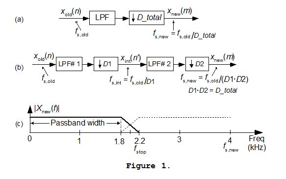
Consider the decimation system in Figure 1(a). When the desired decimation factor D_total is large, say D_total > 20, very significant lowpass filter (LPF) computational savings may be had by implementing the Figure 1(a) single-stage decimation in two stages as shown in Figure 1(b). There we decimate sequence xold(n), whose sample rate is fs,old Hz, by integer factor D1 to produce the intermediate xint(n') sequence. That xint(n') sequence is then decimated by integer factor D2 to yield a final desired sample rate of fs,new Hz. The downsampling, sample rate decrease, operation '↓D1' in Figure 1(b) means discard all but every D1th sample. The product of D1 times D2 is our original desired decimation factor; that is D_total = D1•D2.
Considering Figure 1(b) an important question is, given a desired total downsampling factor D_total, what should be the values of D1 and D2 to minimize the number of taps in lowpass filters LPF# 1 and LP# 2? If for example D_total = 100, should D1•D2 be 5•20, 20•5, 25•4, or maybe 10•10? Thankfully, thoughtful DSP pioneers answered this question for us[1].
An Example:
By way of example, let's assume we have an xold(n) input signal arriving at a sample rate of 400 kHz, and we must decimate that signal by a factor of D_total = 100 to obtain a final sample rate of 4 kHz. Also, let's assume the baseband frequency range of interest is from 0 to 1.8 kHz, and we want 60 dB of filter stopband attenuation. As such, a single-stage-decimation lowpass filter's frequency magnitude response is the solid bold curve shown in Figure 1(c).
So, with fs,new = 4 kHz, we must filter out all xold(n)'s signal energy above fstop by having our filter transition region extend from 1.8 kHz to fstop = 4–1.8 = 2.2 kHz. Using a Figure 1(a) single-stage decimation would require the lowpass filter, LPF, to have roughly 2700 taps. That's a painfully large number! (Resist all temptation to propose using a 2700-tap FIR filter in any system design review meeting at your company, or else you may be forced to update your résumé.)
Good things happen when we partition our decimation operation into two stages. With D_total = 100 in Figure 1(b), the following Matlab code computes the optimum first decimation factor to be D1 = 25, and thus D2 = 4. Using those two-stage decimation factors yields lowpass filters LPF# 1 and LPF# 2 having a total of approximately 200 taps. (Any other combination of the D1 and D2 decimation factors yields lowpass filters having a total of more than 200 taps. For example, had we used D1 = 50 and D2 = 2 (or D1 = 10 and D2 = 10) the total number of two-stage filter taps would have been greater than 250.)
Closing Remarks:
No animals were injured, and no taxpayer money was used, in the preparation of this material

References:
[1] Crochiere, R., and Rabiner, L. "Optimum FIR Digital Implementations for Decimation, Interpolation, and Narrow band Filtering," IEEE Trans. on Acoust. Speech, and Signal Proc., Vol. ASSP 23, No. 5, October 1975.
function [D1,D2] = Dec_OptimTwoStage_Factors(D_Total,Passband_width,Fstop)
%
%    When breaking a single large decimation factor (D_Total) into
%    two stages of decimation (to minimize the orders of the
%    necessary lowpass digital filtering), an optimum first
%    stage of decimation factor (D1) can be found.  The second
%    stage's decimation factor is then D_Total/D1.
%
%    Inputs:
%         D_Total = original single-stage decimation factor.
%         Passband_width = desired passband width of original
%                          single-stage lowpass filter (Hz).
%         Fstop = desired beginning of stopband freq of original
%                          single-stage lowpass filter (Hz).
%
%    Outputs:
%         D1 = optimum first-stage decimation factor.
%         D2 = optimum second-stage decimation factor.
%
%    Example: Assume you want to decimate a sequence by D_Total=100,
%             your original single-stage lowpass filter's passband
%             width and stopband frequency are 1800 and 2200 Hz
%             respectively.  We use:
%
%              [D1,D2] = Dec_OptimTwoStage_Factors(100, 1800, 2200)
%
%             giving us the desired D1 = 25, and D2 = 4.
%             (That is, D1*D2 = 25*4 = 100 = D_Total.)
%
%    Author: Richard Lyons, November, 2011

% Start of processing
    DeltaF = (Fstop -Passband_width)/Fstop;

	Radical = (D_Total*DeltaF)/(2 -DeltaF); % Terms under sqrt sign.
	Numer = 2*D_Total*(1 -sqrt(Radical));  % Numerator.
	Denom = 2 -DeltaF*(D_Total + 1);  % Denominator.
	D1_estimated = Numer/Denom;  %Optimum D1 factor, but not
                                  %                  an integer.

 % Find all factors of 'D_Total'
	Factors_of_D_Total = Find_Factors_of_D_Total(D_Total);

 % Find the one factor of 'D_Total' that's closest to 'D1_estimated'
    Temp = abs(Factors_of_D_Total -D1_estimated);
    Index_of_Min = find(Temp == min(Temp)); % Index of optim. D1
    D1 = Factors_of_D_Total(Index_of_Min); % Optimum first
                                           %    decimation factor
    D2 = D_Total/D1;  % Second decimation factor.

%%%%%%%%%%%%%%%%%%%%%%%%%%%%%%%%%%%%%%%%%%%%%%%%%%%%%%%%%%
function [allfactors] = Find_Factors_of_D_Total(X)
% Finds all integer factors of intger X.
% Filename was originally 'listfactors.m', written
% by Jeff Miller.  Downloaded from Matlab Central.
	[b,m,n] = unique(factor(X));
%b is all prime factors
	occurences = [m(1) diff(m)];
	current_factors = [b(1).^(0:occurences(1))]';
	for index = 2:length(b)
        currentprime = b(index).^(0:occurences(index));
        current_factors = current_factors*currentprime;
        current_factors = current_factors(:);
	end
	allfactors = sort(current_factors);
%%%%%%%%%%%%%%%%%%%%%%%%%%%%%%%%%%%%%%%%%%%%%%%%%%%%%%%%%%


