Delay estimation revisited
Estimates delay and scaling factor between two signals by iteration ( Code snippet: )
Introduction
Quite many DSP-related tasks involve an unknown time delay between signals that needs to be estimated, and maybe corrected. The code snippet presents a "quick-and-dirty" solution - it's not intended for implementation on a DSP, but for testbenches and the like, where robustness and simplicity are more important than efficiency.
The topic is well-researched, for example the references in [1] should be a good starting point.
A Matlab implementation that is stated to be maximum-likelyhood (which would be the "gold standard" for delay estimation) can be found in [2].
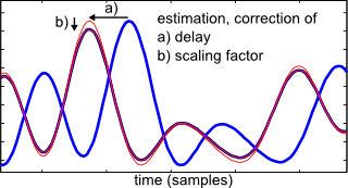
Figure 1 shows an example signal that has been delayed and scaled. The code snippet estimates delay and scaling factor, "un-delays" and scales back so that the output ideally matches the input.
The algorithm is simple but robust. It relies on FFT-based crosscorrelation, for example as illustrated in [3].
More sophisticated frequency domain methods such as [4] are more accurate and efficient, but the difficulty of resolving the +/- pi phase ambiguity may cause them to fail for some input signals, depending on power spectrum and group delay profile. The presented code snippet finds the time delay that maximizes crosscorrelation, regardless of whether "the" delay between the signals over frequency is well-defined or not.
Signals do not need to be coarse-aligned or even arrive in the right order (see "cyclic signals" section below).

Figure 1: delayed / scaled signals
Algorithm
The method isn't particularly imaginative - and that's an advertised feature, as little can go wrong:
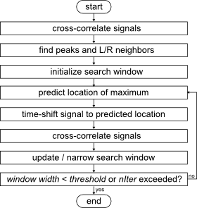
Crosscorrelate, find the highest peak, make an educated guess where the maximum is hiding between the bins, time-shift and repeat.
The flowchart gives a general overview.

Figure 2: Algorithm
The actual iteration loop is somewhat more complex, as finite numerical accuracy gives bitwise identical values of the (shallow) correlation peak over some delay range. If this is observed for two points in the search window, the algorithm will continue to improve the third point, or exit if all three are identical. For a required accuracy up to 10-5 Tsample, this is usually not an issue.
The "educated guess" fits a square polynomial through the three points of the search window and finds the maximum.
After some iterations, numerical accuracy will cause nonsense guesses. If the predicted location of the maximum is outside the search window, it is discarded and linear interpolation is used instead. Otherwise, the algorithm will converge, if slowly.
The polynomial equation is derived here (input file for Maxima computer algebra system (open-source) ).
Methods are known for the interpolation of peaks in FFT data [5], [6] (note, the problem appears similar but is probably not exactly the same). Those could be used to speed up convergence, but I haven't investigated them, as the numerical accuracy of the input data appears to be the main limitation.
Cyclic signals
The signals are treated as cyclic. The first and last sample point have no special meaning, i.e. circshifting both input signals by the same amount will give the same result.
Delaying a signal with sharp transients may reveal ringing that is usually invisible, as long as one stays on the sampling grid:
Nyquist's vestigial sideband theorem [7] promises "no intersample interference", but it keeps quiet about the times between samples...
The delay is returned in the interval [-n/2..n/2], with a signal length of n.
Code snippet
The code snippet includes a demo function that sets up test signals with a known delay. It calls iterDelayEst(...), applies the estimated delay / scaling factor and compares. The result is shown in Figure 3.

Figure 3: Output
Conclusion
The function should return delay and scaling factor to maximize the crosscorrelation, and not be fussy about it.
It's a cleaned-up rewrite, please let me know (comment!) in case of problems.
References
[2] Moddemeijer, R., An information theoretical delay estimator
[4] M. Nentwig: Delay estimation by FFT
[5] R. Lyons: Accurate Measurement of a Sinusoid's Peak Amplitude Based on FFT Data
[6] Tutorial: Interpolating the peak location of a FFT
[7] Lecture notes: Pulse shaping and equalization
% ****************************************************************
% find sub-sample delay and scaling factor between two cyclic signals
% to maximize crosscorrelation
% Markus Nentwig, 120609_v1.1
% ****************************************************************
function iterDelayEstDemo();
    close all;
    n = 1024;
    % n = 1024 * 256; disp('*** test: long signal enabled ***');

    % ****************************************************************
    % random signal
    % ****************************************************************
    fd = randn(1, n) + 1i * randn(1, n);

    % ****************************************************************
    % lowpass filter
    % ****************************************************************
    f = binFreq(n);
    fd(abs(f) > 0.045) = 0;
    s1 = real(ifft(fd)) * sqrt(n);

    % ****************************************************************
    % create delayed 2nd signal
    % ****************************************************************
    dTest_samples = 12.3456;
    cTest = 1.23456;
    % cTest = cTest + 1i; disp('*** test: complex coeff enabled ***');
    % cTest = -cTest; disp('*** test: negative coeff enabled ***');

    s2 = cTest * cs_delay(s1, 1, dTest_samples);
    % s2 = s2 + 0.5*randn(size(s2)); disp('*** test: noise enabled ***');

    % ****************************************************************
    % estimate delay
    % ****************************************************************
    [delay_samples, coeff] = iterDelayEst(s1, s2);

    % ****************************************************************
    % correct it
    % ****************************************************************
    s2a = cs_delay(s1, 1, delay_samples);
    s2b = s2a * coeff;

    figure(); hold on;
    h = plot(real(s1), 'k'); set(h, 'lineWidth', 3);
    h = plot(real(s2), 'b'); set(h, 'lineWidth', 3);
    h = plot(real(s2a), 'r'); set(h, 'lineWidth', 1);
    h = plot(real(s2b), 'm'); set(h, 'lineWidth', 1);
    xlim([1, numel(s1)]);
    xlabel('samples');
    legend('s1', 's2', 's2 un-delayed', 's2 un-delayed and scaled');
    title('test signals');

    format long;
    disp('nominal delay of s2 relative to s1')';
    dTest_samples
    disp('iterDelayEst() returned:');
    delay_samples
    disp('original scaling factor:');
    cTest
    disp('estimated scaling factor:');
    coeff
end

% ****************************************************************
% estimates delay and scaling factor
% ****************************************************************
function [delay_samples, coeff] = iterDelayEst(s1, s2)

    s1 = s1(:) .'; % force row vectors
    s2 = s2(:) .';
    rflag = isreal(s1) && isreal(s2);
    n = numel(s1);
    halfN = floor(n/2);
    assert(numel(s2) == n, 'signals must have same length');

    % ****************************************************************
    % constants
    % ****************************************************************
    % exit if uncertainty below threshold
    thr_samples = 1e-7;

    % exit after fixed number of iterations
    nIter = 25;

    % frequency domain representation of signals
    fd1 = fft(s1);
    fd2 = fft(s2);

    % first round: No delay was applied
    tau = [];
    fd2Tau = fd2; % delayed s2 in freq. domain

    % frequency corresponding to each FFT bin -0.5..0.5
    f = binFreq(n);

    % uncertainty plot data
    e = [];

    % normalization factor
    nf = sqrt((fd1 * fd1') * (fd2 * fd2')) / n; % normalizes to 1

    % search window:
    % known maximum and two surrounding points
    x1 = -1;
    x2 = -1;
    x3 = -1;
    y1 = -1;
    y2 = -1;
    y3 = -1;

    % ****************************************************************
    % iteration loop
    % ****************************************************************
    for count = 1:nIter

        % ****************************************************************
        % crosscorrelation with time-shifted signal
        % ****************************************************************
        xcorr = abs(ifft(fd2Tau .* conj(fd1)))/ nf;

        % ****************************************************************
        % detect peak
        % ****************************************************************
        if isempty(tau)

            % ****************************************************************
            % startup
            % initialize with three adjacent bins around peak
            % ****************************************************************
            ix = find(xcorr == max(xcorr));
            ix = ix(1); % use any, if multiple bitwise identical peaks

            % indices of three bins around peak
            ixLow = mod(ix-1-1, n) + 1; % one below
            ixMid = ix;
            ixHigh = mod(ix-1+1, n) + 1; % one above

            % delay corresponding to the three bins
            tauLow = mod(ixLow -1 + halfN, n) - halfN;
            tauMid = mod(ixMid -1 + halfN, n) - halfN;
            tauHigh = mod(ixHigh -1 + halfN, n) - halfN;

            % crosscorrelation value for the three bins
            xcLow = xcorr(ixLow);
            xcMid = xcorr(ixMid);
            xcHigh = xcorr(ixHigh);

            x1 = tauLow;
            x2 = tauMid;
            x3 = tauHigh;
            y1 = xcLow;
            y2 = xcMid;
            y3 = xcHigh;
        else
            % ****************************************************************
            % only main peak at first bin is of interest
            % ****************************************************************
            tauMid = tau;
            xcMid = xcorr(1);

            if xcMid > y2
                % ****************************************************************
                % improve midpoint
                % ****************************************************************
                if tauMid > x2
                    % midpoint becomes lower point
                    x1 = x2;
                    y1 = y2;
                else
                    % midpoint becomes upper point
                    x3 = x2;
                    y3 = y2;
                end
                x2 = tauMid;
                y2 = xcMid;

            elseif tauMid < x2
                % ****************************************************************
                % improve low point
                % ****************************************************************
                assert(tauMid >= x1); % bitwise identical is OK
                assert(tauMid > x1 || xcMid > y1); % expect improvement
                x1 = tauMid;
                y1 = xcMid;
            elseif tauMid > x2
                % ****************************************************************
                % improve high point
                % ****************************************************************
                assert(tauMid <= x3); % bitwise identical is OK
                assert((tauMid < x3) || (xcMid > y3)); % expect improvement
                x3 = tauMid;
                y3 = xcMid;
            else
                assert(false, '?? evaluated for existing tau ??');
            end
        end

        % ****************************************************************
        % calculate uncertainty (window width)
        % ****************************************************************
        eIter = abs(x3 - x1);
        e = [e, eIter];
        if eIter < thr_samples
            % disp('threshold reached, exiting');
            break;
        end

        if y1 == y2 || y2 == y3
            % reached limit of numerical accuracy on one side
            usePoly = 0;
        else
            % ****************************************************************
            % fit 2nd order polynomial and find maximum
            % ****************************************************************
            num = (x2^2-x1^2)*y3+(x1^2-x3^2)*y2+(x3^2-x2^2)*y1;
            denom = (2*x2-2*x1)*y3+(2*x1-2*x3)*y2+(2*x3-2*x2)*y1;
            if denom ~= 0
                tau = num / denom;
                % is the point within [x1, x3]?
                usePoly = ((tau > x1) && (tau < x3));
            else
                usePoly = 0;
            end
        end
        if ~usePoly
            % revert to linear interpolation on the side with the
            % less-accurate outer sample
            % Note: There is no guarantee that the side with the more accurate
            % outer sample is the right one, as the samples aren't
            % placed on a regular grid!
            % Therefore, iterate to improve the "worse" side, which will
            % eventually become the "better side", and iteration converges.

            tauLow = (x1 + x2) / 2;
            tauHigh = (x2 + x3) / 2;
            if y1 < y3
                o = [tauLow, tauHigh];
            else
                o = [tauHigh, tauLow];
            end
            % don't choose point that is identical to one that is already known
            tau = o(1);
            if tau == x1 || tau == x2 || tau == x3
                tau = o(2);
                if tau == x1 || tau == x2 || tau == x3
                    break;
                end
            end
        end

        % ****************************************************************
        % advance 2nd signal according to location of maximum
        % phase shift in frequency domain - delay in time domain
        % ****************************************************************
        fd2Tau = fd2 .* exp(2i * pi * f * tau);
    end % for

    % ****************************************************************
    % plot the uncertainty (window size) over the number of iterations
    % ****************************************************************
    if true
        figure(); semilogy(e, '+-'); grid on;
        xlabel('iteration');
        title('uncertainty in delay');
    end

    % ****************************************************************
    % the delay estimate is the final location of the delay that
    % maximized crosscorrelation (center of window).
    % ****************************************************************
    delay_samples = x2;

    % ****************************************************************
    % Coefficient: Turn signal 1 into signal 2
    % ****************************************************************
    coeff = fd2Tau * fd1' ./ (fd1 * fd1');

    % ****************************************************************
    % chop roundoff error, if input signals are known to be
    % real-valued.
    % ****************************************************************
    if rflag
        coeff = real(coeff);
    end
end

% ****************************************************************
% frequency corresponding to FFT bin
% ****************************************************************
function f = binFreq(n)
    f = (mod(((0:n-1)+floor(n/2)), n)-floor(n/2))/n;
end

% ****************************************************************
% delay by phase shift
% needed only for demo code
% ****************************************************************
function waveform = cs_delay(waveform, rate_Hz, delay_s)
    rflag = isreal(waveform);

    n = numel(waveform);
    cycLen_s = n / rate_Hz;
    nCyc = delay_s / cycLen_s();

    f = 0:(n - 1);
    f = f + floor(n / 2);
    f = mod(f, n);
    f = f - floor(n / 2);

    phase = -2 * pi * f * nCyc;
    rot = exp(1i*phase);

    waveform = ifft(fft(waveform) .* rot);
    if rflag
        waveform = real(waveform);
    end
end


