Finding the Eigenstructure of A

Starting with the defining equation for an eigenvector $\underline{e}$ and its corresponding eigenvalue $\lambda$ ,

$\displaystyle A\underline{e}_i= \lambda_i \underline{e}_i,\quad i=1,2$

we get

$\displaystyle \left[\begin{array}{cc} c & c-1 \\ [2pt] c+1 & c \end{array}\righ... ...egin{array}{c} \lambda_i \\ [2pt] \lambda_i \eta_i \end{array}\right]. \protect$

(G.23)

We normalized the first element of $\underline{e}_i$ to 1 since $g\underline{e}_i$ is an eigenvector whenever $\underline{e}_i$ is. (If there is a missing solution because its first element happens to be zero, we can repeat the analysis normalizing the second element to 1 instead.)

Equation (G.23) gives us two equations in two unknowns:

$\displaystyle c+\eta_i (c-1)$	$\displaystyle =$	$\displaystyle \lambda_i \protect$	(G.24)
$\displaystyle (1+c) +c\eta_i$	$\displaystyle =$	$\displaystyle \lambda_i \eta_i$	(G.25)

Substituting the first into the second to eliminate $\lambda_i$ , we get

$\begin{eqnarray*} 1+c+c\eta_i &=& [c+\eta_i (c-1)]\eta_i = c\eta_i + \eta_i ^2 (... ...-1)\\ \,\,\Rightarrow\,\,\eta_i &=& \pm \sqrt{\frac{c+1}{c-1}}. \end{eqnarray*}$

Thus, we have found both eigenvectors

$\begin{eqnarray*} \underline{e}_1&=&\left[\begin{array}{c} 1 \\ [2pt] \eta \end{... ...ght], \quad \hbox{where}\\ \eta&\isdef &\sqrt{\frac{c+1}{c-1}}. \end{eqnarray*}$

They are linearly independent provided $\eta\neq0\Leftrightarrow c\neq -1$ and finite provided $c\neq 1$ .

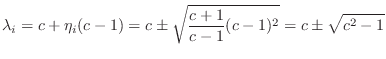
We can now use Eq. $\,$ (G.24) to find the eigenvalues:

$\displaystyle \lambda_i = c + \eta_i (c-1) = c \pm \sqrt{\frac{c+1}{c-1} (c-1)^2} = c \pm \sqrt{c^2-1}$

Assuming $\left\vert c\right\vert<1$ , the eigenvalues are

$\displaystyle \lambda_i = c \pm j\sqrt{1-c^2} \protect$

(G.26)

and so this is the range of

corresponding to sinusoidal oscillation. For $\left\vert c\right\vert>1$ , the eigenvalues are real, corresponding to exponential growth and decay. The values $c=\pm 1$ yield a repeated root (dc or

oscillation).

Let us henceforth assume . In this range $\theta \isdef \arccos(c)$ is real, and we have $c=\cos(\theta)$ , $\sqrt{1-c^2} = \sin(\theta)$ . Thus, the eigenvalues can be expressed as follows:

$\begin{eqnarray*} \lambda_1 &=& c + j\sqrt{1-c^2} = \cos(\theta) + j\sin(\theta)... ...- j\sqrt{1-c^2} = \cos(\theta) - j\sin(\theta) = e^{-j\theta}\\ \end{eqnarray*}$

Equating $\lambda_i$ to $e^{j\omega_i T}$ , we obtain $\omega_i T = \pm \theta$ , or $\omega_i = \pm \theta/T = \pm f_s\theta = \pm f_s\arccos(c)$ , where denotes the sampling rate. Thus the relationship between the coefficient in the digital waveguide oscillator and the frequency of sinusoidal oscillation $\omega$ is expressed succinctly as

$\displaystyle \fbox{$\displaystyle c = \cos(\omega T).$}$

We see that the coefficient range (-1,1) corresponds to frequencies in the range

, and that's the complete set of available digital frequencies.

We have now shown that the system of Fig.G.3 oscillates sinusoidally at any desired digital frequency $\omega$ rad/sec by simply setting $c=\cos(\omega T)$ , where denotes the sampling interval.

Previous: State-Space Analysis Example: The Digital Waveguide Oscillator
Next: Choice of Output Signal and Initial Conditions

Order a Hardcopy of Introduction to Digital Filters

About the Author: Julius Orion Smith III
Julius Smith's background is in electrical engineering (BS Rice 1975, PhD Stanford 1983). He is presently Professor of Music and Associate Professor (by courtesy) of Electrical Engineering at Stanford's Center for Computer Research in Music and Acoustics (CCRMA), teaching courses and pursuing research related to signal processing applied to music and audio systems. See http://ccrma.stanford.edu/~jos/ for details.

Sign in

Search Online Books

Free Online Books

Chapters

See Also

Introduction to Digital Filters
    State Space Filters
       State-Space Analysis Example: The Digital Waveguide Oscillator
          Finding the Eigenstructure of A