


State-Space Analysis Example:
The Digital Waveguide Oscillator
As an example of state-space analysis, we will use it to determine the frequency of oscillation of the system of Fig.G.3 [90].
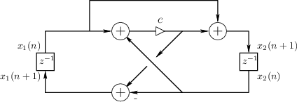
Note the assignments of unit-delay outputs to state variables ![]() and
and ![]() .
From the diagram, we see that
.
From the diagram, we see that
![$\displaystyle \left[\begin{array}{c} x_1(n+1) \\ [2pt] x_2(n+1) \end{array}\rig...
...ay}\right]}_A \left[\begin{array}{c} x_1(n) \\ [2pt] x_2(n) \end{array}\right]
$](http://www.dsprelated.com/josimages_new/filters/img2240.png)
![\begin{eqnarray*}
y_1(n) &\isdef & x_1(n) = [1, 0] {\underline{x}}(n)\\
y_2(n) &\isdef & x_2(n) = [0, 1] {\underline{x}}(n)
\end{eqnarray*}](http://www.dsprelated.com/josimages_new/filters/img2242.png)
A basic fact from linear algebra is that the determinant of a
matrix is equal to the product of its eigenvalues. As a quick
check, we find that the determinant of ![]() is
is
Note that
![]() . If we diagonalize this system to
obtain
. If we diagonalize this system to
obtain
![]() , where
, where
![]() diag
diag![]() ,
and
,
and ![]() is the matrix of eigenvectors of
is the matrix of eigenvectors of ![]() ,
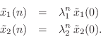
then we have
,
then we have
![$\displaystyle \underline{{\tilde x}}(n) = \tilde{A}^n\,\underline{{\tilde x}}(0...
...t[\begin{array}{c} {\tilde x}_1(0) \\ [2pt] {\tilde x}_2(0) \end{array}\right]
$](http://www.dsprelated.com/josimages_new/filters/img2248.png)
If this system is to generate a real sampled sinusoid at radian frequency
![]() , the eigenvalues
, the eigenvalues ![]() and
and ![]() must be of the form
must be of the form
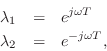
(in either order) where ![]() is real, and
is real, and ![]() denotes the sampling
interval in seconds.
denotes the sampling
interval in seconds.
Thus, we can determine the frequency of oscillation ![]() (and
verify that the system actually oscillates) by determining the
eigenvalues
(and
verify that the system actually oscillates) by determining the
eigenvalues ![]() of
of ![]() . Note that, as a prerequisite, it will
also be necessary to find two linearly independent eigenvectors of
. Note that, as a prerequisite, it will
also be necessary to find two linearly independent eigenvectors of ![]() (columns of
(columns of ![]() ).
).
Finding the Eigenstructure of A
Starting with the defining equation for an eigenvector
![]() and its
corresponding eigenvalue
and its
corresponding eigenvalue ![]() ,
,
![$\displaystyle \left[\begin{array}{cc} c & c-1 \\ [2pt] c+1 & c \end{array}\righ...
...egin{array}{c} \lambda_i \\ [2pt] \lambda_i \eta_i \end{array}\right]. \protect$](http://www.dsprelated.com/josimages_new/filters/img2255.png)
We normalized the first element of
Equation (G.23) gives us two equations in two unknowns:
Substituting the first into the second to eliminate
![\begin{eqnarray*}
1+c+c\eta_i &=& [c+\eta_i (c-1)]\eta_i = c\eta_i + \eta_i ^2 (...
...-1)\\
\,\,\Rightarrow\,\,\eta_i &=& \pm \sqrt{\frac{c+1}{c-1}}.
\end{eqnarray*}](http://www.dsprelated.com/josimages_new/filters/img2261.png)
Thus, we have found both eigenvectors
![\begin{eqnarray*}
\underline{e}_1&=&\left[\begin{array}{c} 1 \\ [2pt] \eta \end{...
...ght], \quad \hbox{where}\\
\eta&\isdef &\sqrt{\frac{c+1}{c-1}}.
\end{eqnarray*}](http://www.dsprelated.com/josimages_new/filters/img2262.png)
They are linearly independent provided
![]() and finite provided
and finite provided ![]() .
.
We can now use Eq.![]() (G.24) to find the eigenvalues:
(G.24) to find the eigenvalues:
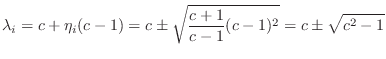
and so this is the range of
Let us henceforth assume
![]() . In this range
. In this range
![]() is real, and we have
is real, and we have
![]() ,
,
![]() . Thus, the eigenvalues can be expressed as follows:
. Thus, the eigenvalues can be expressed as follows:

Equating ![]() to
to
![]() , we obtain
, we obtain
![]() , or
, or
![]() , where
, where ![]() denotes the sampling rate. Thus the
relationship between the coefficient
denotes the sampling rate. Thus the
relationship between the coefficient ![]() in the digital waveguide
oscillator and the frequency of sinusoidal oscillation
in the digital waveguide
oscillator and the frequency of sinusoidal oscillation ![]() is
expressed succinctly as
is
expressed succinctly as
We have now shown that the system of Fig.G.3 oscillates
sinusoidally at any desired digital frequency ![]() rad/sec by simply
setting
rad/sec by simply
setting
![]() , where
, where ![]() denotes the sampling interval.
denotes the sampling interval.
Choice of Output Signal and Initial Conditions
Recalling that
![]() , the output signal from any diagonal
state-space model is a linear combination of the modal signals. The
two immediate outputs
, the output signal from any diagonal
state-space model is a linear combination of the modal signals. The
two immediate outputs ![]() and
and ![]() in Fig.G.3 are given
in terms of the modal signals
in Fig.G.3 are given
in terms of the modal signals
![]() and
and
![]() as
as
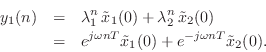
![\begin{eqnarray*}
y_1(n) &=& [1, 0] {\underline{x}}(n) = [1, 0] \left[\begin{arr...
...\lambda_1^n {\tilde x}_1(0) - \eta \lambda_2^n\,{\tilde x}_2(0).
\end{eqnarray*}](http://www.dsprelated.com/josimages_new/filters/img2283.png)
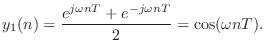
The output signal from the first state variable ![]() is
is
The initial condition
![]() corresponds to modal initial
state
corresponds to modal initial
state
![$\displaystyle \underline{{\tilde x}}(0) = E^{-1}\left[\begin{array}{c} 1 \\ [2p...
...nd{array}\right] = \left[\begin{array}{c} 1/2 \\ [2pt] 1/2 \end{array}\right].
$](http://www.dsprelated.com/josimages_new/filters/img2286.png)
Next Section:
References
Previous Section:
Repeated Poles


