


Single-Input, Single-Output (SISO) FDN
When there is only one input signal ![]() , the input vector
, the input vector
![]() in Fig.2.28 can be defined as the scalar input
in Fig.2.28 can be defined as the scalar input ![]() times a
vector of gains:
times a
vector of gains:
![\includegraphics[width=\twidth]{eps/FDNSISO}](http://www.dsprelated.com/josimages_new/pasp/img555.png)
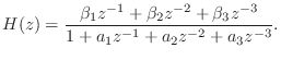
Note that when
![]() , this system is capable of realizing
any transfer function of the form
, this system is capable of realizing
any transfer function of the form
The more general case shown in Fig.2.29 can be handled in one of
two ways: (1) the matrices
![]() can be augmented
to order
can be augmented
to order
![]() such that the three delay lines are replaced
by
such that the three delay lines are replaced
by ![]() unit-sample delays, or (2) ordinary state-space analysis
may be generalized to non-unit delays, yielding
unit-sample delays, or (2) ordinary state-space analysis
may be generalized to non-unit delays, yielding
![$\displaystyle \mathbf{D}(z) \isdef \left[\begin{array}{ccc} z^{-M_1} & 0 & 0\\ [2pt] 0 & z^{-M_2} & 0\\ [2pt] 0 & 0 & z^{-M_3} \end{array}\right]. \protect$](http://www.dsprelated.com/josimages_new/pasp/img539.png)
In FDN reverberation applications,
![]() , where
, where
![]() is an orthogonal matrix, for reasons addressed below, and
is an orthogonal matrix, for reasons addressed below, and
![]() is a
diagonal matrix of lowpass filters, each having gain bounded by 1. In
certain applications, the subset of orthogonal matrices known as
circulant matrices have advantages [385].
is a
diagonal matrix of lowpass filters, each having gain bounded by 1. In
certain applications, the subset of orthogonal matrices known as
circulant matrices have advantages [385].
Next Section:
FDN Stability
Previous Section:
FDN and State Space Descriptions


