Model Signal Impairments at Complex Baseband

• Matlab
• Tutorials

In this article, we develop complex-baseband models for several signal impairments: interfering carrier, multipath, phase noise, and Gaussian noise.  To provide concrete examples, we’ll apply the impairments to a QAM system. The impairment models are Matlab functions that each use at most seven lines of code.  Although our example system is QAM, the models can be used for any complex-baseband signal.

I used a very simple complex-baseband model of a QAM system in my last post to show how to compute the modulation error ratio (MER) [1].  This article uses a similar QAM system model.

Figure 1 is a simplified block diagram of a QAM system.  The transmitter includes a source of QAM symbols, a root-Nyquist pulse-shaping filter, and a Quadrature modulator.  The receiver has a Quadrature downconverter, root-Nyquist filter, and decision block.  The wide lines represent complex (I/Q) signals, and the narrow lines represent the real modulated signal.  We refer to the I/Q signals as complex-baseband signals [2].  The matched root-Nyquist filters perform the dual tasks of limiting the bandwidth of the transmitted signal while minimizing the interference from other symbols at the sampling instant [3,4].  For our purpose of modeling impairments, I have left out the usual key receiver systems of AGC, carrier recovery, clock recovery, and adaptive equalization.

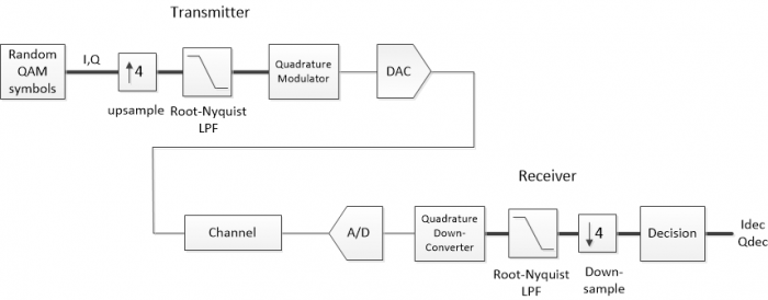
Figure 1.  Simplified QAM system block diagram.

We’ll model the channel at complex baseband, so we can eliminate the Quadrature up and down conversions.  This is more efficient than modeling the modulated signal, because the sample rate need only be greater than 2X the I/Q signal bandwidth, rather than 2X the frequency of the modulated signal.  Since we’ll model the entire system as discrete-time, the D/A and A/D converters will be left out.  We then have the block diagram of Figure 2.  Again, keep in mind that this model does not include any clock or carrier error, and has no clock or carrier recovery loops.  It is useful for modeling linear impairments, but it is not valid for some nonlinear impairments, for example clipping of the modulated signal.  I have created two Matlab functions for the transmitter and receiver, qam_tx.m and qam_rx.m.  These are listed in Appendix A of the attached PDF document.  Matlab functions for the different channel impairment cases are listed in Appendix B of the PDF document.  Their names are shown underneath the “Channel Impairments” block in Figure 2.

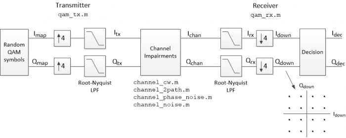
Figure 2.  Simplified QAM system at complex baseband.

Figure 3 plots some of the labeled signals from Figure 2 for a QAM-16 system impaired by Gaussian noise.  The plots were generated using qam_tx.m, channel_noise.m, and a modified version of qam_rx.m (see section 4 below for details).  Figure 3a shows the random QAM symbols as a Q_map vs I_map constellation plot.  The spectrum of the transmitted signal I_tx/Q_tx is plotted in Figure 3b.  Figure 3c is an eyeplot of the output of the receiver’s root-Nyquist filter, I_rx.  At this point, the signal has 4 samples per symbol, so the valid sampling instants are spaced 4 samples apart.  For our simplified model, the eye opening aligns exactly with every fourth sample (A real-world receiver must compute the correct sample value using a variable interpolator).  The eyes are partially closed due to the noise added to the signal.  Downsampling I_rx and Q_rx by 4 at the correct sample alignment gives the symbol-rate signals I_down and Q_down, who’s constellation plot is shown in Figure 3d.  The noise is visible as “fuzz” around the nominal constellation points.

Now we’ll develop the complex-baseband impairment models and see how they affect QAM signals.  Matlab code for the impairment models is listed in Appendix B of the PDF document.  In the following, the function qam_rx.m plots the constellation Q_down vs. I_down and also computes MER.

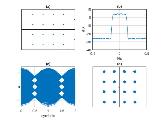
Figure 3.  Signals from Figure 2 for QAM-16 modulation with added noise.

a. I_map/Q_map constellation  b. I_chan/Q_chan spectrum   c. I_rx eyeplot  d. I_down/Q_down constellation

1.  Interfering Carrier Model

At complex baseband, a sinusoidal signal with magnitude A and frequency ω₀ is represented as:

$$ A exp(j\omega_0nT_s)= A cos(\omega_0nT_s)+jAsin(\omega_0nT_s)  $$

Where n is sample index and T_s is sample time.  To model an interfering carrier, we simply add this signal to I_tx/Q_tx (see Figure 4):

$$ I_{chan}= I_{tx}+A cos(\omega_0nT_s)  \qquad  \qquad $$

$$ Q_{chan}= Q_{tx}+A sin(\omega_0nT_s)  \qquad (1)$$

Equation 1 is implemented by the Matlab function channel_cw.m, which is listed in Appendix B of the PDF document (cw stands for continuous wave).  The following code creates a QAM-64 signal, adds an interfering carrier, and plots the receiver constellation.  It also computes the carrier-to-interference ratio (C/I).  For this example, the interferer amplitude A = 0.25, f₀= 14 Hz, and f_s= 100 Hz.

    M= 64;                     % constellation order
    N= 8192;                   % number of symbols
    [Itx,Qtx]= qam_tx(M,N);    % create complex baseband QAM signal
    A= .25;                    % interferer amplitude
    f0= 14;                    % Hz inteferer freq
    fs= 100;                   % Hz sample freq
    [Ichan,Qchan]= channel_cw(Itx,Qtx,A,f0,fs);    % add interferer
    % compute C/I
    Psig = sum(Itx.^2 + Qtx.^2)/(4*N);     % avg. signal power
    Pint= A.^2;                            % interferer power
    CtoI= 10*log10(Psig/Pint)
    % simplified QAM RX – plot constellation
    qam_rx(M,Ichan,Qchan)

The spectrum of I_chan + j*Q_chan is plotted in figure 5, showing the interferer at 14 Hz.  The asymmetry of the complex spectrum should come as no surprise.  The C/I ratio is computed as:

CtoI =10.2304 dB

The QAM constellation plotted by qam_rx.m is shown in Figure 6.  Here, the interference is visible as a circle around each constellation point.  The radius of the circle is equal to the amplitude of the sinusoidal interferer after filtering by the receiver’s root-Nyquist filter.  In this example, the interferer results in received signal MER of 22.3 dB.  This is not equal to the C/I at the receiver input, because the interferer at 14 Hz is attenuated by the receiver’s filter.

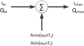
Figure 4.  Complex-baseband channel model for interfering carrier.

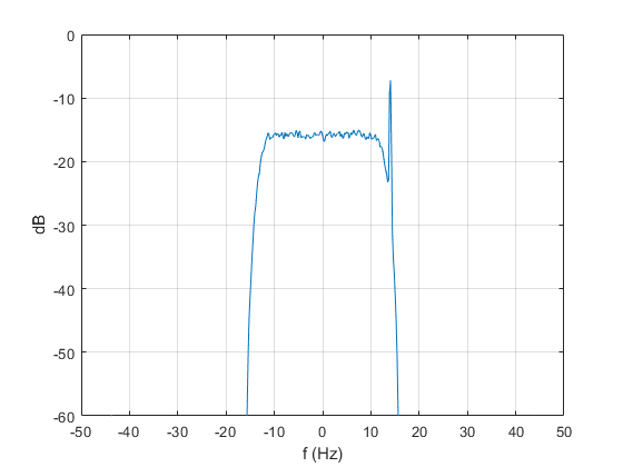
Figure 5.  Spectrum of I_chan + j*Q_chan showing interfering carrier at 14 Hz.

            y= Ichan + j*Qchan;
            [P,f]= pwelch(y,hanning(512),256,512,fs);
            P= fftshift(P);            % shift center freq to 0 Hz
            f= f- fs/2;                % shift center freq to 0 Hz
            PdB= 10*log10(P);          % dB psd estimate
            plot(f,PdB),grid

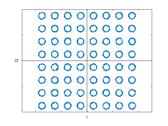
Figure 6. QAM-64 constellation plot of Q_down vs I_down with interfering carrier.          

2.  Multipath Model

Multipath occurs when a signal follows more than one path to the receiver.  The multiple paths have different delay, amplitude, and phase, with possible time-variation of these parameters.  The channel can be described by a main path with gain of 1.0, plus one or more paths with different delay, amplitude and phase with respect to the main path.  The multipath channel transfer function can be written as:

$$ H(\omega)= 1+b_1exp(-j\omega T_1)+b_2exp(-j\omega T_2) + ... \qquad (2) $$

where the b_i are complex and the T_i are the (continuous-time) delays of each path with respect to the main path.  In order to model multipath as a sampled system, we assume $T_1 \approx kT_s,\ T_2 \approx mT_s $, etc., where k and m are integers.  (If this assumption is not accurate for a given system, the sample rate of the model can be increased to make T_s << T_i). Then, substituting z= exp(jωT_s) into Equation 2, we get:

$$ H(z)= 1+b_1z^{-k}+b_2z^{-m}+ ... \qquad (3) $$

H(z) looks familiar – it is just the transfer function of an FIR filter (with b₀ = 1).  The filter coefficients are complex.  The number of taps depends on the longest delay T_max:  N_taps = round(T_max/T_s) + 1.  Only the taps that match a path delay receive non-zero coefficients.

The simplest multipath system has two paths:  a two-path model at complex baseband is shown in Figure 7.  Here, b₁ = Ae^jφ and the multiplier is full-complex.  For a two-path model, only the first and last taps are nonzero.

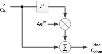
Figure 7.  Complex-baseband channel model for two-path.              

2.1  Multipath Channel Response

Let’s look at the response of a two-path channel when the input is a unit impulse.  For this example, we’ll use the fixed parameters A = 0.15, φ = π/3, and k = 5 samples.  We will use the Matlab function channel_2path.m to implement a complex FIR filter based on these parameters (see Appendix B of the PDF document).  Here is the code to find the channel output I_chan/Q_chan:

    A= 0.15;                  % amplitude of 2nd path
    phi= pi/3;                % rad phase of 2nd path
    k= 5;                     % samples delay of 2nd path
    % find channel impulse response
    Itx= [0 1 0 0 0 0];       % impulse input
    Qtx= [0 0 0 0 0 0];
    [Ichan,Qchan]= channel_2path(Itx,Qtx,k,A,phi);

The real and imaginary parts of the channel’s impulse response are plotted in Figure 8 a and b.  The magnitude response is shown in Figure 8c.  The channel has an amplitude ripple of roughly 2.5 dB.  The delay response is plotted in Figure 8d:  Delay ripple is roughly 1.5 samples.  Magnitude and Delay responses were computed as follows:

    fs= 1;
    y= Ichan + j*Qchan;
    [h,f]= freqz(y,1,256,'whole',fs);
    H= 20*log10(abs(h));                    % Magnitude response, dB
    H= fftshift(H);                         % shift center freq to 0 Hz
    [D,f]= grpdelay(y,1,256,'whole',fs);    % group delay in samples
    D= fftshift(D);                         % shift center freq to 0 Hz
    f= f- fs/2;                             % shift center freq to 0 Hz

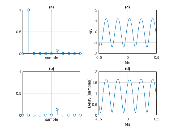
Figure 8.  Multipath Channel Response

a. Real part of impulse response   b. Imaginary part of impulse response

c. Magnitude response   d. Group Delay

2.2  QAM-16 signal applied to a multipath channel

Using the same channel parameters as above, we’ll look at how the two-path channel affects a complex-baseband QAM-16 signal.  The QAM signal has 4 samples per symbol, so the multipath delay k of 5 samples equals 1.25 QAM symbol times.  Here is the code to generate the QAM signal, apply it to the channel, and plot the receiver constellation:

    A= 0.15;                   % amplitude of 2nd path
    phi= pi/3;                 % rad phase of 2nd path
    k= 5;                      % samples delay of 2nd path
    M= 16;                     % constellation order
    N= 8192;                   % number of symbols
    [Itx,Qtx]= qam_tx(M,N);    % create complex baseband QAM signal
    [Ichan,Qchan]= channel_2path(Itx,Qtx,k,A,phi);    % 2-path channel model
    qam_rx(M,Ichan,Qchan)         % simplified QAM RX -- plot constellation

The Spectrum of the QAM signal I_chan + j*Q_chan at the output of the channel model is shown in Figure 9.  Consistent with the magnitude response of Figure 8c, the channel has produced about 2.5 dB of amplitude ripple.  The QAM constellation plotted by qam_rx.m is shown in Figure 10.  The inter-symbol interference (ISI) caused by multipath is pronounced.  Note the tilt of the cloud around each constellation point depends on the phase angle of the second path.  A signal with narrower bandwidth would suffer less delay variation and thus less ISI.  For example, a multi-carrier QAM system such as Orthogonal Frequency Division Multiplexing with its narrow subcarriers is less sensitive to multipath, and requires only a simple scaling of amplitude and phase of each subcarrier to adapt to the channel.

In modeling multipath, we typically don’t know precise or even approximate values of amplitude and delay.  We just have estimates of the range of these parameters.  The parameters can be set to arbitrary values over their ranges, which allows testing receiver subsystems such as adaptive equalizers.

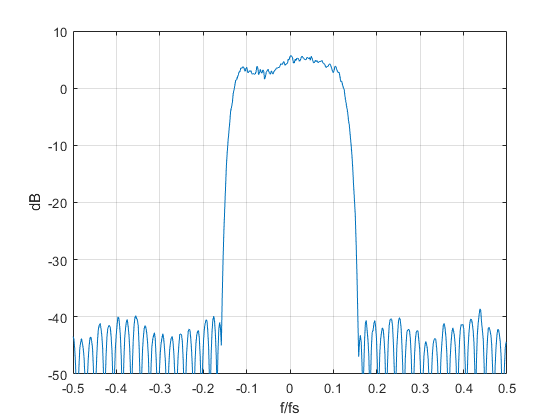
Figure 9.  Spectrum of QAM signal at output of 2-path channel.

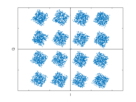
Figure 10.  QAM-16 Constellation plot of Q_down vs I_down for 2-path channel.

3.  Phase Noise Model

Oscillator phase noise (time jitter) can be random or periodic, and can be transferred to the signal in various ways.  Two common sources are the transmitter DAC sample clock and receiver ADC sample clock.   Also, if the transmitter or receiver use mixers, any phase noise on the local oscillators will be transferred to the signal.  Although you could say that phase noise occurs in the transmitter or receiver rather than in the channel, it is convenient to create a channel model for phase noise.

To add phase noise φ to a complex baseband signal I_tx/Q_tx, we just multiply by e^jφ :

$$ I_{chan}+ jQ_{chan}= (I_{tx}+jQ_{tx})e^{j\phi} $$

The block diagram for the model is shown in Figure 11.  For our examples, we will use sinusoidal phase noise:

$$ \phi(n)= \phi_{max}cos(\omega_0 nT_s) \qquad radians$$

Where φ_max is peak phase deviation in radians.  The Matlab function channel_phase_noise.m implements the complex baseband model for phase noise (see Appendix B of the PDF document).

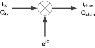
Figure 11.  Complex-baseband channel model for phase noise.

3.1  Adding phase noise to a fixed signal vector

Suppose every sample from a complex-baseband transmitter has the fixed value of [I_tx, Q_tx] = [5/8, 5/8].  In other words, every sample is at the same constellation point of [5/8, 5/8].  (If this constant-value signal is then quadrature modulated, the transmitted signal is a sinusoid).  Let’s add phase noise of peak amplitude π/20 radians and frequency of 3 Hz to this signal.  Let the sample frequency equal 100 Hz.  Here is the Matlab code for adding the phase noise:

    N= 1024;                % number of samples
    Itx= 5/8*ones(1,N);     % fixed constellation point
    Qtx= 5/8*ones(1,N);
    phi_max= pi/20;         % rad peak phase deviation
    f0= 3;                  % Hz phase modulation frequency
    fs= 100;                % Hz sample frequency
    [Ichan,Qchan]= channel_phase_noise(Itx,Qtx,phi_max,f0,fs);

Q_chan vs. I_chan is plotted in Figure 12.  The phase excursion of the blue trace is +/- π/20 radians.  The spectrum of the signal with phase noise is shown in Figure 13.  Phase modulation sidebands appear at multiples of 3 Hz.

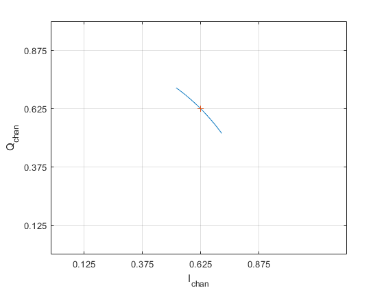
Figure 12.  Sinusoidal phase noise added to fixed signal vector [I_tx, Q_tx] = [5/8, 5/8].

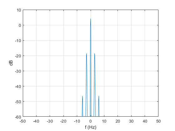
Figure 13.  Spectrum of I_chan + j*Q_chan with sinusoidal phase noise.

3.2  QAM-64 signal with added phase noise

Now we’ll add sinusoidal phase noise to a QAM-64 signal.  The sample rate and noise frequency are the same as used in the previous example.  Peak amplitude of the noise is .06 radians.  The Matlab code to generate the complex-baseband signal, add phase noise, and plot the receiver constellation is as follows:

    M= 64;                      % constellation order
    N= 8192;                    % number of symbols
    [Itx,Qtx]= qam_tx(M,N);     % create complex baseband QAM signal
    phi_max= .06;               % rad peak phase deviation
    f0= 3;                      % Hz phase modulation frequency
    fs= 100;                    % Hz sample frequency
    [Ichan,Qchan]= channel_phase_noise(Itx,Qtx,phi_max,f0,fs);
    qam_rx(M,Ichan,Qchan)         % simplified QAM RX – plot constellation

The constellation plot of the received QAM-64 signal is shown in Figure 14.  Like what we saw in Figure 12, the phase noise causes the symbols to be spread over arcs, with the worst spreading on the outer constellation points.  For high constellation orders, it is important that phase noise be controlled.  Otherwise, it can cause too many symbol errors on the outer constellation points.

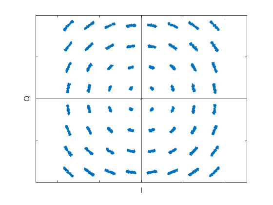
Figure 14.  QAM-64 constellation plot of Q_down vs I_down with added phase noise.

4.  Gaussian Noise Model

The Matlab function channel_noise.m implements a complex baseband model for Gaussian noise (see Appendix B of the PDF document).  It simply adds Gaussian noise to the I and Q signals:

    Ichan= Itx + sigma/sqrt(2)*randn(1,L);
    Qchan= Qtx + sigma/sqrt(2)*randn(1,L);

Here, sigma is the standard deviation of the noise and the noise added to the Q channel is independent of that added to the I channel.  L is the length of the input signal vectors I_tx and Q_tx.  The channel model is shown in Figure 15.

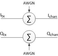
Figure 15.  Complex-baseband channel model for Gaussian noise.

Here is the Matlab code to add Gaussian noise to a QAM-16 signal:

    M= 16;                          % constellation order
    N= 8192;                        % number of symbols
    [Itx,Qtx]= qam_tx(M,N);         % create complex baseband QAM signal
    sigma= .05;                     % noise standard deviation
    [Ichan,Qchan]= channel_noise(Itx,Qtx,sigma);    % add noise
    qam_rx(M,Ichan,Qchan)            % simplified QAM RX – plot constellation

The spectrum of I_chan + j*Q_chan is plotted in Figure 3b, and the receiver QAM constellation is shown in Figure 3d.  The function qam_rx.m computes the MER of the signal as 29.7 dB.  This is approximately equal to the level of the signal density relative to noise density in Figure 3b.

5.  Summary

We have presented a few complex-baseband channel models for signal impairments.  For the case of a QAM signal, our very simple receiver model allowed us to use the received constellation plot to diagnose impairments.  We have seen that an interfering carrier creates rings around the constellation points, and phase noise creates arcs that are most pronounced on the outer points.  Multipath creates a cloud of ISI on each constellation point.  (Note:  unlike our simple receiver model, a typical QAM receiver would include an adaptive equalizer to compensate for multipath).

Impairments can also harm receiver functions that we have not modeled; for example, the carrier recovery and clock recovery subsystems.  Severe impairments can prevent lock of the carrier recovery or clock recovery loops.

Finally, you can cascade channel models to explore the effect of multiple impairments.  For example, the constellation for a QAM-16 signal with both Gaussian noise and interfering carrier is shown in Figure 16, along with the Matlab code involved.

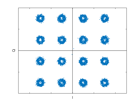
Figure 16.  QAM-16 constellation plot of Q_down vs I_down with interfering carrier and Gaussian noise.

    M= 16; N= 8192;
    [Itx,Qtx]= qam_tx(M,N);         % create complex baseband QAM signal
    Anoise= .05;                    % noise standard deviation
    [I1,Q1]= channel_noise(Itx,Qtx,Anoise);    % add noise
    Acw= .25;                       % interferer amplitude
    f0= 14;                         % Hz inteferer freq
    fs= 100;                        % Hz sample freq
    [Ichan,Qchan]= channel_cw(I1,Q1,Acw,f0,fs);    % add interferer
    qam_rx(M,Ichan,Qchan)           % simplified QAM RX – plot constellation

References

1.  Robertson, Neil, “Compute Modulation Error Ratio (MER) for QAM”, DSP Related, Nov, 2019.

https://www.dsprelated.com/showarticle/1305.php

2.  William H. Tranter, et. al., Communication Systems Simulation, Prentice Hall, 2004, section 4.1.1.

3.  Rice, Michael, Digital Communications, Pearson, 2009, Section A.2.

4.  Course Notes EE4061, “Intersymbol Interference/Nyquist Pulse Shaping”, Georgia Institute of Technology, 2011. 

http://wireless-systems.ece.gatech.edu/4601/lectures-2011/week10.pdf

Neil Robertson           December, 2019     Revised section 3 12/19/19

Sign in