Compute Modulation Error Ratio (MER) for QAM

• Matlab
• Tutorials

This post defines the Modulation Error Ratio (MER) for QAM signals, and shows how to compute it.  As we’ll see, in the absence of impairments other than noise, the MER tracks the signal’s Carrier-to-Noise Ratio (over a limited range).  A Matlab script at the end of the PDF version of this post computes MER for a simplified QAM-64 system.

Figure 1 is a simplified block diagram of a QAM system.  The transmitter includes a source of QAM symbols, a root-Nyquist pulse-shaping filter and a Quadrature modulator.  The receiver has a Quadrature downconverter, root-Nyquist filter, and decision block.  The wide lines represent complex (I/Q) signals, and the narrow lines represent the real modulated signal.  The matched root-Nyquist filters perform the dual tasks of limiting the bandwidth of the transmitted signal while minimizing the interference from other symbols at the sampling instant [1,2].  For our discussion of MER, I have left out the usual key receiver systems of AGC, carrier recovery, clock recovery, and adaptive equalization.

This article is available in PDF format for easy printing.

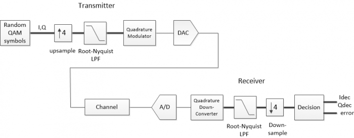
Figure 1.  Simplified QAM system block diagram.

For our purposes, we can model the channel at complex baseband [3], so we can eliminate the Quadrature up and down conversions.  Also, we will model the entire system as discrete-time, so the D/A and A/D converters can be left out.  We then have the block diagram of Figure 2a, where the channel includes Gaussian noise (AWGN) added to I and Q, plus a block labeled “other impairments”.  These could include linear impairments such as multipath, phase noise, and interference.  In this article, our focus is on noise, so we’ll leave out the other impairments.

Figure 3 plots some of the labeled signals from Figure 2 for a QAM-16 system with noise.  Figure 3a shows the random QAM symbols as a Q_map vs I_map constellation plot.  Figure 3b is an eyeplot of the output of the receiver’s root-Nyquist filter, I_rx.  At this point, the signal has 4 samples per symbol, so the valid sampling instants are spaced 4 samples apart.  For our simplified model, the eye opening aligns exactly with every fourth sample (A real-world receiver must compute the correct sample value using a variable interpolator).  The eyes are partially closed due to the noise added to the signal.  Downsampling I_rx and Q_rx by 4 at the correct sample alignment gives I_down and Q_down, who’s constellation plot is shown in Figure 3c.  The noise is visible as “fuzz” around the nominal constellation points.  The final outputs I_dec and Q_dec are computed in the decision block by rounding (slicing) I_down and Q_down to the nearest allowed symbol value, reproducing the original transmitter constellation (Figure 3d).

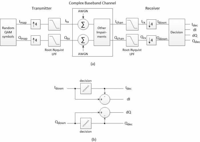
Figure 2.  Simplified QAM system at complex baseband.

a. Overall block diagram.  AWGN:  additive white Gaussian noise.

b.  Decision block.  dI= I_down – I_dec; dQ= Q_down – Q_dec

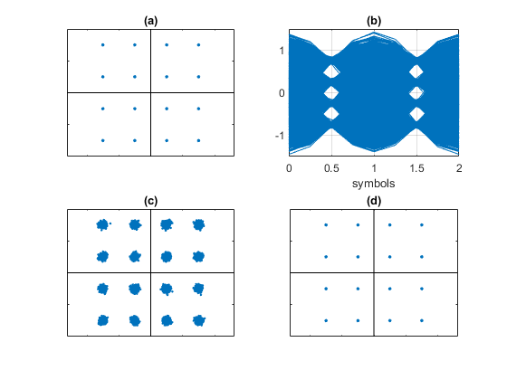
Figure 3.  Signals from Figure 2 for QAM-16 modulation with added noise.

a. I_map/Q_map constellation  b. I_rx eyeplot  c. I_down/Q_down constellation  d. I_dec/Q_dec constellation

MER Formula

The Modulation Error Ratio is a way to quantify the constellation noise seen in Figure 3c.  Figure 4 shows the QAM-16 symbols Q_dec vs I_dec at the output of the decision block.  Also shown is a single received symbol of I_down/Q_down at the input of the decision block.  The modulation error ratio of this single symbol is defined as:

$$ MER\; (one \,symbol) = \frac{I_{dec}^2+Q_{dec}^2}{dI^2+dQ^2}$$

Where dI and dQ are the errors with respect to the target symbol I_dec/Q_dec.  In words, MER is the ratio of the target symbol power to the error power.  dI and dQ are computed as shown in the block diagram of the decision block (Figure 2b):  dI = I_down – I_dec; dQ = Q_down – Q_dec.

If N symbols are received, the MER is defined as the average:

$$MER= \frac1{N}\sum_{i=1}^N\frac{I_{dec}(i)^2+Q_{dec}(i)^2}{dI(i)^2+dQ(i)^2}$$

If N is large and all symbols are equally likely, we can calculate MER as the ratio of average target symbol power to average error power [4]:

$$MER= \frac{avg. target\,symbol\,power}{avg. error\,power} \qquad $$

$$=\frac{\frac1{N}\sum_{i=1}^NI_{dec}(i)^2 +Q_{dec}(i)^2}{\frac1{N}\sum_{i=1}^NdI(i)^2+dQ(i)^2} \qquad(1)$$

For a given constellation order, the numerator is a constant – call it P_av:

$$MER=\frac{P_{av}}{\frac1{N}\sum_{i=1}^NdI(i)^2+dQ(i)^2} \qquad(2)$$

Since P_av is a constant, we don’t have to evaluate it over all of the received symbols.  Instead, we can find P_av by evaluating the numerator of Equation 1 over N = 4 constellation points in the first quadrant of QAM-16.  For a square constellation, we’ll use I and Q from the set +/- k/M^1/2, where k is odd and M is constellation order.  For M= 16, the set is +/- {1/4, 3/4}, and the constellation points in the first quadrant are 

$(\frac14,\frac14) ;(\frac14,\frac34);(\frac34,\frac14);(\frac34,\frac34).$  The average constellation power of QAM-16 is thus:

$$P_{av}\;(QAM16)= \frac14*( (\frac14)^2 + (\frac14)^2  + (\frac14)^2 + (\frac34)^2$$

$$+ (\frac34)^2  + (\frac14)^2 + (\frac34)^2 + (\frac34)^2 ) = \frac58 $$

We can write the MER in dB as:

$$ MER \;(dB)=10log_{10}P_{av} - 10log_{10}\left(\frac1N\sum_{i=1}^N dI(i)^2+dQ(i)^2\right) \qquad(3)$$

If noise is the only signal impairment, and if matched (root-Nyquist) filters are used in transmitter and receiver, the MER can equal the signal’s carrier-to-noise ratio (C/N).  In reality, accurate estimation of C/N is only possible over a limited range.  The maximum MER is limited by impairments of the transmitter and receiver themselves.  The low end is also limited:  when C/N is low enough to cause symbol errors, the calculated MER loses accuracy.  This occurs because each decision error causes the error power calculation for that symbol to be too low.  When there are many errors, the calculated MER will be too high.

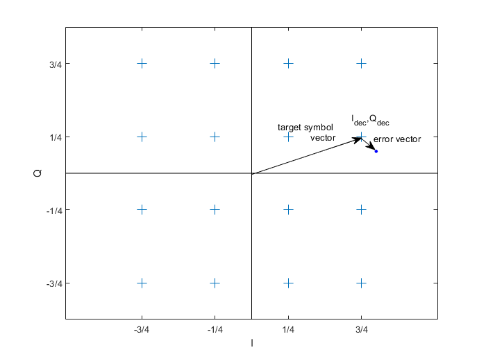
Figure 4.  QAM-16 constellation points (symbols), with target signal vector and error vector.

Example

This example computes MER of a QAM-64 signal with added noise.  Matlab code that implements the simplified QAM system is listed in the PDF version of this post.  As shown in Figure 2a, Gaussian noise is added to the I and Q channels.  Figure 5a shows the spectrum of I_chan + jQ_chan, which has a C/N of about 30 dB.  An eyeplot of the receiver signal I_rx is shown in Figure 5b.  The receiver constellation is shown in Figure 5c, along with the value of MER calculated by Equation 3.  As expected, the calculated MER matches the C/N.  

In calculating MER for QAM-64, we used P_av = 21/32 = -1.83 dB.  The I and Q values of QAM-64 come from the set +/- {1/8 3/8 5/8 7/8}.  The root-Nyquist filters used have excess bandwidth α = 0.25.  This gives an occupied signal bandwidth of 1.25*f_symbol = 1.25*f_s/4 = .3125 f_s (Figure 5a).

A convenient way to calculate the average error power is to filter dI² + dQ² using a one-pole IIR filter.  The output of the filter can be used to compute a running estimate of MER, as shown in Figure 5d.

Finally, Figure 6 shows the receive constellation with no noise added to the transmitted signal.  The MER of 41 dB is a measure of the Inter-symbol interference (ISI) [1,2] of the cascaded transmit and receive root-Nyquist filters in our simplified model.

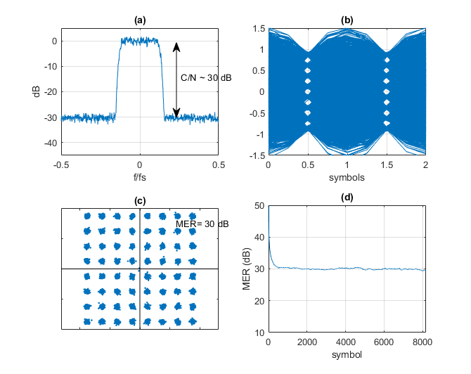
Figure 5.  QAM-64 Model Outputs

a.  Spectrum at RX input, showing added noise.  b.  Eyeplot of I_rx

c.  Receiver constellation plot.  d.  MER calculated by filtering dI² + dQ² using a one-pole IIR filter.

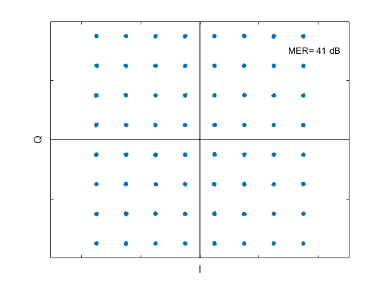
Figure 6.  Receive Constellation with no noise added to the transmitted signal.        

References

1.  Rice, Michael, Digital Communications, Pearson, 2009, Section A.2.

2.  Course Notes EE4061, “Intersymbol Interference/Nyquist Pulse Shaping”, Georgia Institute of Technology, 2011.  http://wireless-systems.ece.gatech.edu/4601/lectures-2011/week10.pdf

3.  William H. Tranter, et. al., Communication Systems Simulation, Prentice Hall, 2004, section 4.1.1.

4.  Cisco Systems, “Digital Transmission:  Carrier-to-Noise Ratio, Signal-to-Noise Ratio, and Modulation Error Ratio”, 2006. 

 http://www.mdmit.pl/apps/mdmit/download/Mibs%20for%20cable%20modems/Hi_res_CNR-SNR_WP_1115b.pdf

Neil Robertson     November, 2019       revised 4/17/20

Sign in