Design Square-Root Nyquist Filters

In his book on multirate signal processing, harris presents a nifty technique for designing square-root Nyquist FIR filters with good stopband attenuation [1].  In this post, I describe the method and provide a Matlab function for designing the filters.  You can find a Matlab function by harris for designing the filters at [2].

Background

Single-carrier modulation, such as QAM, uses filters to limit the bandwidth of the signal.  Figure 1 shows a simplified QAM system block diagram with I and Q filters in the transmitter and receiver.  The impulse response of the filters generally has ringing that causes inter-symbol interference, or ISI, between the transmitted symbols.  We can limit the ISI by judicious filter design.  It turns out that a filter with a frequency response as shown in Figure 2a has theoretically zero ISI.  This so-called Nyquist filter [3] has a magnitude response of 0.5 at f_symbol/2, and the response is odd-symmetric about f_symbol/2.  It also must have linear phase.  The stopband edge is at:

$$f= (1+\alpha)\frac{f_{symbol}}{2},\qquad 0<\alpha<1 \qquad (1) $$

Given that the minimum bandwidth to transmit a symbol sequence is f_symbol/2, the parameter α is called the excess bandwidth.

Figure 2b plots the impulse response of a Nyquist filter that has four samples per transmitted symbol.  The samples that occur at symbol intervals are shown in red.  As desired, all of these samples other than the center one are near zero (near zero ISI).

We could place I and Q Nyquist filters in the transmitter, and everything would work fine … except for noise.  For optimal performance with noise, the receive filter must have a response that is a time-reversed version of the transmit filter [4,5].  For symmetrical filters, this means the transmit and receive filters must have identical impulse responses, i.e., they must be matched filters.  How can we achieve zero ISI with matched filters?  In the frequency domain, the matched filter response H(f) must satisfy:

$$ |H(f)|\cdot|H(f)|= |H_{nyquist}(f)| $$

where H_nyquist(f) is the response of a Nyquist filter.  We then have:

$$|H(f)|= |H_{nyquist}(f)|^{1/2} \qquad (2) $$

H(f) is called a square-root Nyquist response.  Figure 3 plots a square-root Nyquist response and a “full” Nyquist response (dashed).  As shown, the response of the square-root Nyquist filter at f_symbol/2 is the square-root of 0.5, or -3.01 dB.  Besides providing optimal noise performance, the square-root Nyquist response in the receive filter allows for good adjacent-channel rejection.

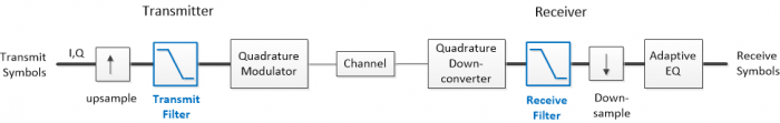
Figure 1.  QAM Transmitter and Receiver Simplified Block Diagram.  Wide lines = complex (I/Q).

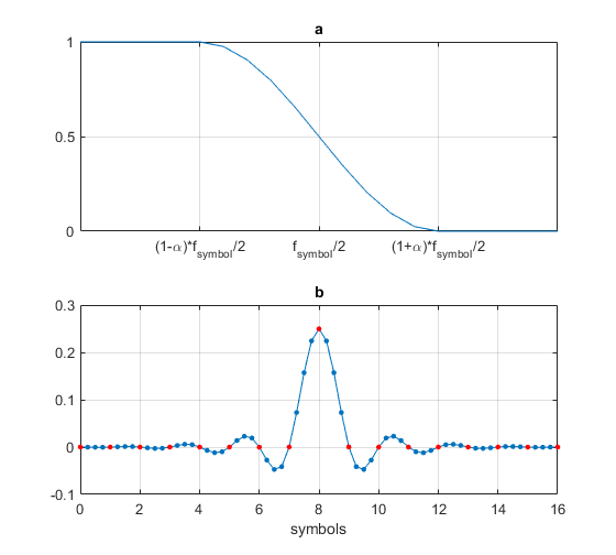
Figure 2.  a) Nyquist filter magnitude response (linear amplitude scale).

                b) Impulse response of a Nyquist filter with 4 samples per symbol.

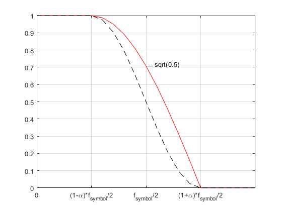
Figure 3.  Square-root Nyquist magnitude response (in red), linear amplitude scale.

A Matlab function to design square-root Nyquist FIR filters

Appendix A in the PDF version lists the Matlab function root_nyq.m for designing square-root Nyquist FIR filters.  It is based on the technique presented in reference [1].  The function uses the Matlab Parks-McClellan filter design function firpm, with stopband edge of (1 + α)*f_symbol/2.  The strategy is to find a passband edge frequency f_pass that results in:

$$|H(f_{symbol}/2)|=\sqrt{1/2}\qquad(3) $$

as shown in Figure 3.  A gradient search is performed over f_pass, and a new filter is synthesized for each f_pass value, until the goal response is met with acceptable error.

Note that using f_pass= (1 - α)*f_symbol/2 results in a response of 0.5 at f_symbol/2, which exceeds the attenuation goal.  Thus, this value of f_pass is always below the desired value.  It is convenient to start the search at this frequency, with each step adjusting the value of f_pass until the error in the response is minimized.  

Even though the function optimizes the transition band response at just one frequency, ISI is quite good.  And, for a given number of taps, filters designed using root_nyq.m have much higher stopband attenuation than square-root raised cosine (SRRC) filters [1].

Example 1

In root_nyq.m, symbol time T_symbol has units of samples.  For this example, let T_symbol = 4 samples and excess bandwidth alpha = 0.25.  Then, to design a 65-tap filter, we use the following Matlab code, which also computes the filter’s magnitude response, assuming sample rate of 200Hz:

    ntaps= 65;
    Tsymbol= 4;                % samples  symbol time
    alpha= .25;                % excess bandwidth
    b= root_nyq(ntaps,Tsymbol,alpha);
    fs= 200;
    [h,f]= freqz(b,1,512,fs);
    H= 20*log10(abs(h));

The magnitude response is plotted in Figure 4.  Given 4 samples per symbol, f_symbol = f_s/4 = 50 Hz, and f_symbol/2 = f_s/8 = 25 Hz.  As desired, the response is -3 dB at 25 Hz.  The stopband edge is at (1 + alpha)*f_symbol/2 = 1.25*25 = 31.25 Hz.

Next, we’ll display an eyeplot of random binary symbols for the cascade of two identical square-root Nyquist filters.  The following code generates random binary data, upsamples by four, and applies the upsampled signal to the cascade of two filters.

    b_full= conv(b,b);           % cascade two root-nyquist filters
    N= 1024;                     % number of symbols
    u= round(rand(1,N));
    x= u -1/2;                   % binary symbols at 1 sample/symbol
    x_up= zeros(1,4*N);
    x_up(1:4:4*N)= 4*x;          % upsample to 4 samples/symbol
    y= filter(b_full,1,x_up);    % apply x_up to full-Nyquist filter
    eyeplot(y(65:end),Tsymbol),xlabel('symbols')

The eyeplot is shown in figure 5 (The function eyeplot.m is listed in Appendix B of the PDF version).  Note that it is allowable to have transmit and receive square-root Nyquist filters with different numbers of taps.  However, in simulations, it is then sometimes necessary to resample the receive filter output to get optimal ISI.

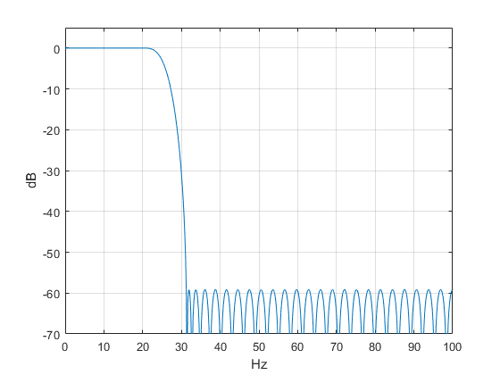
Figure 4.  Square-root Nyquist filter magnitude response, ntaps= 65, f_s= 200 Hz, f_symbol/2 = 25 Hz, and alpha= 0.25.

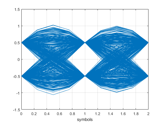
Figure 5.  Eyeplot at output of cascaded square-root Nyquist filters (T_symbol = 4 samples).

Example 2

Let T_symbol = 2 samples, ntaps = 42 and excess bandwidth alpha = 0.2.  The Matlab code to design the square-root Nyquist filter is as follows:

    ntaps= 42;
    Tsymbol= 2;
    alpha= .2;
    b= root_nyq(ntaps,Tsymbol,alpha);

The magnitude response is plotted in Figure 6, where we have again assumed sample frequency of 200 Hz.  f_symbol/2 = 50 Hz and stopband edge is 1.2*50 = 60 Hz.

As in example 1, we can find the eyeplot for the cascade of two identical square-root Nyquist filters using random binary symbols.  As a way to quantify the ISI, we will also compute the Modulation Error Ratio (MER) of the cascaded filters, assuming BPSK modulation.  I described MER calculation in an earlier post [6].  The Matlab code is as follows:

    b_full= conv(b,b);             % cascade two root-nyquist filters
    % generate eye plot
    N= 1024;                       % number of symbols
    u= round(rand(1,N));
    x= u -1/2;                     % random symbols at 1 sample/symbol
    x_up= zeros(1,2*N);
    x_up(1:2:2*N)= 2*x;            % upsample to 2 samples/symbol
    y= filter(b_full,1,x_up);      % apply x_up to full-Nyquist filter
    eyeplot(y(62:end),Tsymbol),xlabel('symbols'),figure
    
    % compute MER of BPSK due to root-Nyquist ISI
    Pavg= -6.02;                   % dB avg power of constellation [-.5 .5]
    I= y(62:2:end);                % decimate to one sample/symbol
    dI= abs(I) - .5;               % error
    e_sq= dI.^2;                   % error squared
    e_sq_avg= sum(e_sq)/length(I);
    mer_dB= Pavg - 10*log10(e_sq_avg)

The eyeplot is shown in Figure 7.  The MER varies slightly depending on the random symbol sequence, and is approximately 51 dB.  We can compute MER for several values of ntaps – the result is plotted, along with stopband attenuation, in Figure 8.  ntaps should be chosen to achieve MER that puts minimal stress on the forward error correction algorithm.  If an adaptive equalizer is used, it may be able to adapt to achieve MER greater than that of the cascaded matched filters.

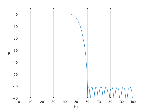
Figure 6.  Square-root Nyquist filter magnitude response, ntaps= 42, f_s= 200 Hz, f_symbol/2 = 50 Hz, and alpha= 0.2.

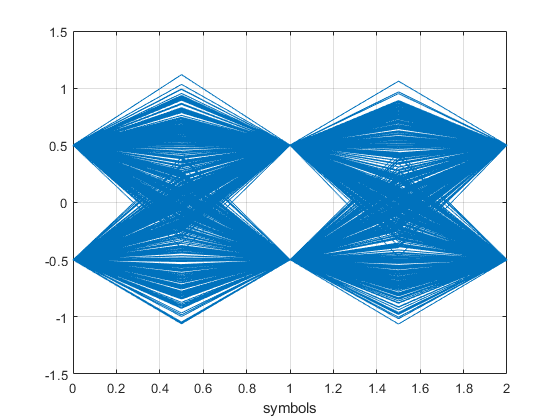
Figure 7.  Eyeplot at output of cascaded square-root Nyquist filters (T_symbol = 2 samples).

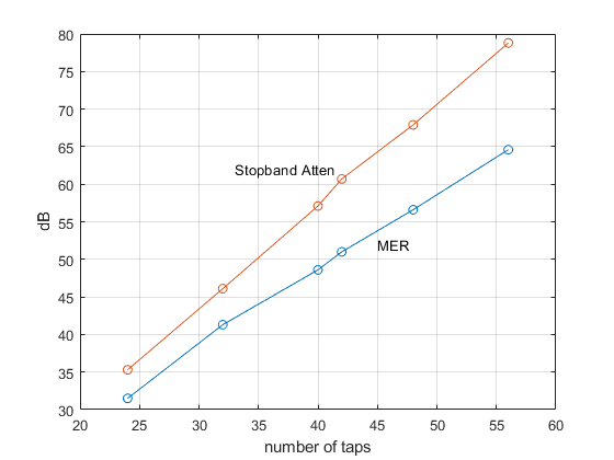
Figure 8.  MER and Stopband Attenuation vs. ntaps for alpha= 0.2 and T_symbol = 2 samples.

See PDF version for Appendix A and B.

References

1.  harris, fredric j., Multirate Signal Processing for Communications Systems, Prentice Hall, 2004, section 4.3.2

2.  Website for reference 1, https://www.informit.com/store/multirate-signal-processing-for-communication-systems-9780131465114

3.  Rice, Michael, Digital Communications, A Discrete-Time Approach, Pearson, 2009, section A.2

4.  harris, p 86-88.

5.  Sklar, Bernard, Digital Communications:  Fundamentals and Applications, Prentice Hall, 1988, section 2.9.2.

6.  Robertson, Neil, “Compute Modulation Error Ratio (MER) for QAM", dspRelated.com, Nov., 2019, https://www.dsprelated.com/showarticle/1305.php

7.  Rice, section A.2.3.

Neil Robertson     July, 2020                       

Sign in