


Matlab Filter Implementation
In this section, we will implement (in matlab) the simplest lowpass filter
- Fig.1.3 listed simplp for filtering one block of data, and
- Fig.1.4 listed a main program for testing simplp.
y = filter (B, A, x)
where
- x is the input signal (a vector of any length),
- y is the output signal (returned equal in length to x),
- A is a vector of filter feedback coefficients, and
- B is a vector of filter feedforward coefficients.
where
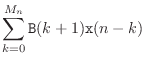
Note that Eq.![]() (2.1) could be written directly in matlab using two
for loops (as shown in Fig.3.2). However, this
would execute much slower because the matlab language is
interpreted, while built-in functions such as filter
are pre-compiled C modules. As a general rule, matlab programs should
avoid iterating over individual samples whenever possible. Instead,
whole signal vectors should be processed using expressions involving
vectors and matrices. In other words, algorithms should be
``vectorized'' as much as possible.
Accordingly, to get the most out of matlab, it is necessary to know
some linear algebra [58].
(2.1) could be written directly in matlab using two
for loops (as shown in Fig.3.2). However, this
would execute much slower because the matlab language is
interpreted, while built-in functions such as filter
are pre-compiled C modules. As a general rule, matlab programs should
avoid iterating over individual samples whenever possible. Instead,
whole signal vectors should be processed using expressions involving
vectors and matrices. In other words, algorithms should be
``vectorized'' as much as possible.
Accordingly, to get the most out of matlab, it is necessary to know
some linear algebra [58].
The simplest lowpass filter of Eq.![]() (1.1) is nonrecursive
(no feedback), so the feedback coefficient vector A is set to
1.3.5 Recursive filters will be
introduced later in §5.1. The minus sign in
Eq.
(1.1) is nonrecursive
(no feedback), so the feedback coefficient vector A is set to
1.3.5 Recursive filters will be
introduced later in §5.1. The minus sign in
Eq.![]() (2.1) will make sense after we study
filter transfer functions in Chapter 6.
(2.1) will make sense after we study
filter transfer functions in Chapter 6.
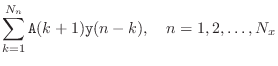
The feedforward coefficients needed for the simplest lowpass filter are
With these settings, the filter function implements
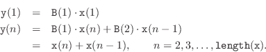
% simplpm1.m - matlab main program implementing
%              the simplest lowpass filter:
%
%                    y(n) = x(n)+x(n-1)}

N=10;       % length of test input signal
x = 1:N;    % test input signal (integer ramp)
B = [1,1];  % transfer function numerator
A = 1;      % transfer function denominator

y = filter(B,A,x);

for i=1:N
  disp(sprintf('x(%d)=%f\ty(%d)=%f',i,x(i),i,y(i)));
end

% Output:
%   octave:1> simplpm1
%   x(1)=1.000000       y(1)=1.000000
%   x(2)=2.000000       y(2)=3.000000
%   x(3)=3.000000       y(3)=5.000000
%   x(4)=4.000000       y(4)=7.000000
%   x(5)=5.000000       y(5)=9.000000
%   x(6)=6.000000       y(6)=11.000000
%   x(7)=7.000000       y(7)=13.000000
%   x(8)=8.000000       y(8)=15.000000
%   x(9)=9.000000       y(9)=17.000000
%   x(10)=10.000000     y(10)=19.000000
|
A main test program analogous to Fig.1.4 is shown in Fig.2.1. Note that the input signal is processed in one big block, rather than being broken up into two blocks as in Fig.1.4. If we want to process a large sound file block by block, we need some way to initialize the state of the filter for each block using the final state of the filter from the preceding block. The filter function accommodates this usage with an additional optional input and output argument:
[y, Sf] = filter (B, A, x, Si)
Si denotes the filter initial state, and
Sf denotes its final state. A main program illustrating
block-oriented processing is given in Fig.2.2.
% simplpm2.m - block-oriented version of simplpm1.m

N=10;       % length of test input signal
NB=N/2;     % block length
x = 1:N;    % test input signal
B = [1,1];  % feedforward coefficients
A = 1;      % feedback coefficients (no-feedback case)

[y1, Sf] = filter(B,A,x(1:NB));      % process block 1
      y2 = filter(B,A,x(NB+1:N),Sf); % process block 2

for i=1:NB   % print input and output for block 1
  disp(sprintf('x(%d)=%f\ty(%d)=%f',i,x(i),i,y1(i)));
end

for i=NB+1:N % print input and output for block 2
  disp(sprintf('x(%d)=%f\ty(%d)=%f',i,x(i),i,y2(i-NB)));
end
|
Next Section:
Simulated Sine-Wave Analysis in Matlab
Previous Section:
Elementary Filter Theory Problems


