


Taylor Series with Remainder
We repeat the derivation of the preceding section, but this time we treat the error term more carefully.
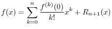
Again we want to approximate ![]() with an
with an ![]() th-order polynomial:
th-order polynomial:
Our problem is to find
![]() so as to minimize
so as to minimize
![]() over some interval
over some interval ![]() containing
containing ![]() . There are many
``optimality criteria'' we could choose. The one that falls out
naturally here is called Padé approximation. Padé
approximation sets the error value and its first
. There are many
``optimality criteria'' we could choose. The one that falls out
naturally here is called Padé approximation. Padé
approximation sets the error value and its first ![]() derivatives to
zero at a single chosen point, which we take to be
derivatives to
zero at a single chosen point, which we take to be ![]() . Since all
. Since all
![]() ``degrees of freedom'' in the polynomial coefficients
``degrees of freedom'' in the polynomial coefficients ![]() are
used to set derivatives to zero at one point, the approximation is
termed maximally flat at that point. In other words, as
are
used to set derivatives to zero at one point, the approximation is
termed maximally flat at that point. In other words, as
![]() , the
, the ![]() th order polynomial approximation approaches
th order polynomial approximation approaches ![]() with an error that is proportional to
with an error that is proportional to ![]() .
.
Padé approximation comes up elsewhere in signal processing. For example, it is the sense in which Butterworth filters are optimal [53]. (Their frequency responses are maximally flat in the center of the pass-band.) Also, Lagrange interpolation filters (which are nonrecursive, while Butterworth filters are recursive), can be shown to maximally flat at dc in the frequency domain [82,36].
Setting ![]() in the above polynomial approximation produces
in the above polynomial approximation produces
Differentiating the polynomial approximation and setting ![]() gives
gives
In the same way, we find
From this derivation, it is clear that the approximation error (remainder
term) is smallest in the vicinity of ![]() . All degrees of freedom
in the polynomial coefficients were devoted to minimizing the approximation
error and its derivatives at
. All degrees of freedom
in the polynomial coefficients were devoted to minimizing the approximation
error and its derivatives at ![]() . As you might expect, the approximation
error generally worsens as
. As you might expect, the approximation
error generally worsens as ![]() gets farther away from 0.
gets farther away from 0.
To obtain a more uniform approximation over some interval ![]() in
in ![]() , other kinds of error criteria may be employed. Classically,
this topic has been called ``economization of series,'' or simply
polynomial approximation under different error criteria. In
Matlab or
Octave, the function
polyfit(x,y,n) will find the coefficients of a polynomial
, other kinds of error criteria may be employed. Classically,
this topic has been called ``economization of series,'' or simply
polynomial approximation under different error criteria. In
Matlab or
Octave, the function
polyfit(x,y,n) will find the coefficients of a polynomial ![]() of
degree n that fits the data y over the points x in a
least-squares sense. That is, it minimizes
of
degree n that fits the data y over the points x in a
least-squares sense. That is, it minimizes

Next Section:
Formal Statement of Taylor's Theorem
Previous Section:
Informal Derivation of Taylor Series


