


2D Mesh and the Wave Equation
 |
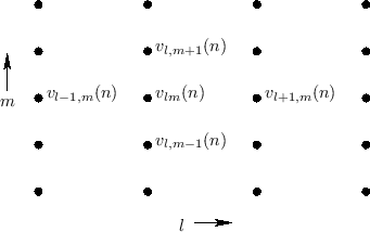
Consider the 2D rectilinear mesh, with nodes at positions ![]() and
and
![]() , where
, where ![]() and
and ![]() are integers, and
are integers, and ![]() and
and ![]() denote the
spatial sampling intervals along
denote the
spatial sampling intervals along ![]() and
and ![]() , respectively
(see Fig.C.33).
Then from
Eq.
, respectively
(see Fig.C.33).
Then from
Eq.![]() (C.105) the junction velocity
(C.105) the junction velocity ![]() at time
at time ![]() is given
by
is given
by
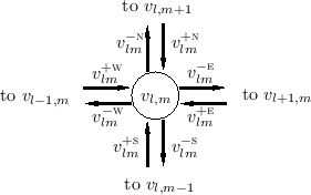
These incoming traveling-wave components arrive from the four
neighboring nodes after a one-sample propagation delay. For example,
![]() , arriving from the north, departed from node
, arriving from the north, departed from node
![]() at time
at time ![]() , as
, as
![]() .
Furthermore, the outgoing components at time
.
Furthermore, the outgoing components at time
![]() will arrive at the neighboring nodes
one sample in the future at time
will arrive at the neighboring nodes
one sample in the future at time ![]() .
For example,
.
For example,
![]() will become
will become
![]() .
Using these relations, we can
write
.
Using these relations, we can
write
![]() in terms of the four outgoing waves from its
neighbors at time
in terms of the four outgoing waves from its
neighbors at time ![]() :
:
where, for instance,
This may be shown in detail by writing
![\begin{eqnarray*}
v_{lm}(n-1)
&=& \frac{1}{2}[v_{lm}^{+\textsc{n}}(n-1) + \cdot...
...}^{-\textsc{n}}(n-1) + \cdots + v_{lm}^{-\textsc{w}}(n-1)\right]
\end{eqnarray*}](http://www.dsprelated.com/josimages_new/pasp/img4027.png)
so that
![\begin{eqnarray*}
v_{lm}(n-1)
&=& \frac{1}{2}[v_{lm}^{-\textsc{n}}(n-1) + \cdot...
...
v_{l,m-1}^{+\textsc{n}}(n) +
v_{l-1,m}^{+\textsc{e}}(n)\right].
\end{eqnarray*}](http://www.dsprelated.com/josimages_new/pasp/img4028.png)
Adding Equations (C.116-C.116), replacing
terms such as
![]() with
with
![]() , yields a computation in terms of physical node velocities:
, yields a computation in terms of physical node velocities:
![\begin{eqnarray*}
\lefteqn{v_{lm}(n+1) + v_{lm}(n-1) = } \\
& & \frac{1}{2}\left[
v_{l,m+1}(n) +
v_{l+1,m}(n) +
v_{l,m-1}(n) +
v_{l-1,m}(n)\right]
\end{eqnarray*}](http://www.dsprelated.com/josimages_new/pasp/img4031.png)
Thus, the rectangular waveguide mesh satisfies this equation
giving a formula for the velocity at node ![]() , in terms of
the velocity at its neighboring nodes one sample earlier, and itself
two samples earlier. Subtracting
, in terms of
the velocity at its neighboring nodes one sample earlier, and itself
two samples earlier. Subtracting
![]() from both sides yields
from both sides yields
![\begin{eqnarray*}
\lefteqn{v_{lm}(n+1) - 2 v_{lm}(n) + v_{lm}(n-1)} \\
&=& \fra...
.... \left[v_{l+1,m}(n) - 2 v_{lm}(n) + v_{l-1,m}(n)\right]\right\}
\end{eqnarray*}](http://www.dsprelated.com/josimages_new/pasp/img4033.png)
Dividing by the respective sampling intervals, and assuming ![]() (square mesh-holes), we obtain
(square mesh-holes), we obtain
![\begin{eqnarray*}
\lefteqn{\frac{v_{lm}(n+1) - 2 v_{lm}(n) + v_{lm}(n-1)}{T^2}} ...
...ft.\frac{v_{l+1,m}(n) - 2 v_{lm}(n) + v_{l-1,m}(n)}{X^2}\right].
\end{eqnarray*}](http://www.dsprelated.com/josimages_new/pasp/img4035.png)
In the limit, as the sampling intervals ![]() approach zero such that
approach zero such that
![]() remains
constant, we recognize these expressions as the definitions of the partial
derivatives with respect to
remains
constant, we recognize these expressions as the definitions of the partial
derivatives with respect to ![]() ,
, ![]() , and
, and ![]() , respectively, yielding
, respectively, yielding
![$\displaystyle \frac{\partial^2 v(t,x,y)}{\partial t^2} = \frac{X^2}{2T^2}
\left...
...^2 v(t,x,y)}{\partial x^2}
+ \frac{\partial^2 v(t,x,y)}{\partial y^2}
\right].
$](http://www.dsprelated.com/josimages_new/pasp/img4038.png)
![$\displaystyle \frac{\partial^2 v}{\partial t^2} =
c^2
\left[
\frac{\partial^2 v}{\partial x^2}
+ \frac{\partial^2 v}{\partial y^2}
\right]
$](http://www.dsprelated.com/josimages_new/pasp/img4040.png)
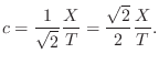
Discussion regarding solving the 2D wave equation subject to boundary conditions appears in §B.8.3. Interpreting this value for the wave propagation speed
Next Section:
The Lossy 2D Mesh
Previous Section:
Recent Developments


