Time-Varying Delay-Line Reads
If denotes the input to a time-varying delay, the output can be
written as
![$\displaystyle y(t)=x(t-D_t).
$](http://www.dsprelated.com/josimages_new/pasp/img1268.png)
![$ D_t$](http://www.dsprelated.com/josimages_new/pasp/img1269.png)
![$ x(t-D_t)$](http://www.dsprelated.com/josimages_new/pasp/img1270.png)
Let's analyze the frequency shift caused by a time-varying delay by
setting to a complex sinusoid at frequency
:
![$\displaystyle x(t) = e^{j\omega_s t}
$](http://www.dsprelated.com/josimages_new/pasp/img1271.png)
![$\displaystyle y(t)= x(t-D_t) = e^{j\omega_s \cdot (t-D_t)}.
$](http://www.dsprelated.com/josimages_new/pasp/img1272.png)
![$\displaystyle \theta(t)= \angle y(t) = \omega_s \cdot(t-D_t)
$](http://www.dsprelated.com/josimages_new/pasp/img1273.png)
where
![$ \omega_l $](http://www.dsprelated.com/josimages_new/pasp/img1250.png)
![$ {\dot D_t}\isdef \frac{d}{dt}D_t$](http://www.dsprelated.com/josimages_new/pasp/img1275.png)
![$ D_t$](http://www.dsprelated.com/josimages_new/pasp/img1269.png)
![$ {\dot D_t}$](http://www.dsprelated.com/josimages_new/pasp/img1276.png)
![$\displaystyle {\dot D_t}= \frac{\omega_s -\omega_l }{\omega_s }.
$](http://www.dsprelated.com/josimages_new/pasp/img1277.png)
Comparing Eq.(5.6) to Eq.
(5.2), we find that the
time-varying delay most naturally simulates Doppler shift caused by a
moving listener, with
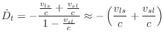
That is, the delay growth-rate,
![$ {\dot D_t}$](http://www.dsprelated.com/josimages_new/pasp/img1276.png)
![$ c$](http://www.dsprelated.com/josimages_new/pasp/img125.png)
Simulating source motion is also possible, but the relation
between delay change and desired frequency shift is more complex, viz.,
from Eq.(5.2) and Eq.
(5.6),
![$\displaystyle {\dot D_t}= - \frac{\frac{v_{ls}}{c} + \frac{v_{sl}}{c}}{1-\frac{v_{sl}}{c}}
\approx - \left(\frac{v_{ls}}{c} + \frac{v_{sl}}{c}\right)
$](http://www.dsprelated.com/josimages_new/pasp/img1279.png)
![$ v_{sl}\ll c$](http://www.dsprelated.com/josimages_new/pasp/img1280.png)
The time-varying delay line was described in §5.1. As discussed there, to implement a continuously varying delay, we add a ``delay growth parameter'' g to the delayline function in Fig.5.1, and change the line
rptr += 1; // pointer updateto
rptr += 1 - g; // pointer updateWhen g is 0, we have a fixed delay line, corresponding to
![$ {\dot D_t}=0$](http://www.dsprelated.com/josimages_new/pasp/img1281.png)
![$ \,$](http://www.dsprelated.com/josimages_new/pasp/img196.png)
![$ \texttt{g}>0$](http://www.dsprelated.com/josimages_new/pasp/img1228.png)
![$ \texttt{g}$](http://www.dsprelated.com/josimages_new/pasp/img1229.png)
![$ {\dot D_t}=\texttt{g}$](http://www.dsprelated.com/josimages_new/pasp/img1230.png)
![$ \,$](http://www.dsprelated.com/josimages_new/pasp/img196.png)
![$\displaystyle \texttt{g} = -\frac{v_{ls}}{c}
$](http://www.dsprelated.com/josimages_new/pasp/img1282.png)
![$ v_{ls}$](http://www.dsprelated.com/josimages_new/pasp/img1251.png)
Note that when the read- and write-pointers are driven directly from a model of physical propagation-path geometry, they are always separated by predictable minimum and maximum delay intervals. This implies it is unnecessary to worry about the read-pointer passing the write-pointers or vice versa. In generic frequency shifters [275], or in a Doppler simulator not driven by a changing geometry, a pointer cross-fade scheme may be necessary when the read- and write-pointers get too close to each other.
Next Section:
Multiple Read Pointers
Previous Section:
Doppler Simulation via Delay Lines