


Ideal Spectral Interpolation
Ideally, the spectrum of any signal ![]() at any frequency
at any frequency
![]() is obtained by projecting the signal
is obtained by projecting the signal ![]() onto the
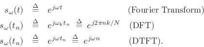
zero-phase, unit-amplitude, complex sinusoid at frequency
onto the
zero-phase, unit-amplitude, complex sinusoid at frequency ![]() [264]:
[264]:
 |
(3.43) |
where
Thus, for signals in the DTFT domain which are time limited to
![]() ,
we obtain
,
we obtain
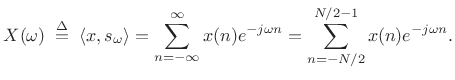 |
(3.44) |
This can be thought of as a zero-centered DFT evaluated at
Next Section:
Interpolating a DFT
Previous Section:
Spectral Roll-Off


