


Filters Preserving Phase
In this chapter, linear phase and zero phase filters are defined and discussed.
Linear-Phase Filters
(Symmetric Impulse Responses)
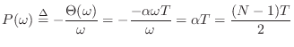
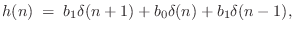
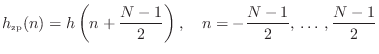
A linear-phase filter is typically used when a causal filter is needed to modify a signal's magnitude-spectrum while preserving the signal's time-domain waveform as much as possible. Linear-phase filters have a symmetric impulse response, e.g.,
We will show that every real symmetric impulse response corresponds to
a real frequency response times a
linear phase term
![]() , where
, where
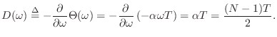
![]() is the slope of the linear phase. Linear phase is
often ideal because a filter phase of the form
is the slope of the linear phase. Linear phase is
often ideal because a filter phase of the form
![]() corresponds to phase delay
corresponds to phase delay
Zero-Phase Filters
(Even Impulse Responses)
A zero-phase filter is a special case of a linear-phase filter
in which the phase slope is ![]() . The real impulse response
. The real impulse response
![]() of a zero-phase filter is even.11.1 That is, it satisfies
of a zero-phase filter is even.11.1 That is, it satisfies
A zero-phase filter cannot be causal (except in the trivial
case when the filter is a constant scale factor
![]() ).
However, in many ``off-line'' applications, such as when filtering a
sound file on a computer disk, causality is not a requirement, and
zero-phase filters are often preferred.
).
However, in many ``off-line'' applications, such as when filtering a
sound file on a computer disk, causality is not a requirement, and
zero-phase filters are often preferred.
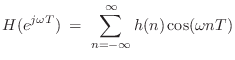
It is a well known Fourier symmetry that real, even signals have real, even Fourier transforms [84]. Therefore,
This follows immediately from writing the DTFT of
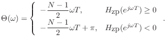
A real frequency response has phase zero when it is positive, and
phase ![]() when it is negative. Therefore, we define
a zero-phase filter as follows:
when it is negative. Therefore, we define
a zero-phase filter as follows:

Recall from §7.5.2 that a passband is defined as a
frequency band that is ``passed'' by the filter, i.e., the filter is
not designed to minimize signal amplitude in the band. For example,
in a lowpass filter with cut-off frequency ![]() rad/s, the
passband is
rad/s, the
passband is
![]() .
.
 -Phase Filters
Under our definition, a zero-phase filter always has a real, even
impulse response [
![]() ], but not every real, even, impulse
response is a zero-phase filter. For example, if
], but not every real, even, impulse
response is a zero-phase filter. For example, if ![]() is zero
phase, then
is zero
phase, then ![]() is not; however, we could call
is not; however, we could call ![]() a
``
a
``![]() -phase filter'' if we like (a zero-phase filter in series with
a sign inversion).
-phase filter'' if we like (a zero-phase filter in series with
a sign inversion).
Phase in the Stopband
Practical zero-phase filters are zero-phase in their passbands, but
may switch between 0 and ![]() in their stopbands (as illustrated in
the upcoming example of Fig.10.2). Thus, typical zero-phase
filters are more precisely described as piecewise constant-phase
filters, where the constant phase is 0 in all passbands, and
in their stopbands (as illustrated in
the upcoming example of Fig.10.2). Thus, typical zero-phase
filters are more precisely described as piecewise constant-phase
filters, where the constant phase is 0 in all passbands, and ![]() over various intervals within stopbands. Similarly, practical
``linear phase'' filters are typically truly linear phase across their
passbands, but typically exhibit discontinuities by
over various intervals within stopbands. Similarly, practical
``linear phase'' filters are typically truly linear phase across their
passbands, but typically exhibit discontinuities by ![]() radians in their
stopband(s). As long as the stopbands are negligible, which is the
goal by definition, the
radians in their
stopband(s). As long as the stopbands are negligible, which is the
goal by definition, the ![]() -phase regions can be neglected
completely.
-phase regions can be neglected
completely.
Example Zero-Phase Filter Design
Figure 10.1 shows the impulse response and frequency response of a length 11 zero-phase FIR lowpass filter designed using the Remez exchange algorithm.11.2 The matlab code for designing this filter is as follows:
N = 11;                % filter length - must be odd
b = [0 0.1 0.2 0.5]*2; % band edges
M = [1  1   0   0 ];   % desired band values
h = remez(N-1,b,M);    % Remez multiple exchange design
The impulse response h is returned in linear-phase form, so it must be left-shifted
![\includegraphics[width=\twidth ]{eps/remezexa}](http://www.dsprelated.com/josimages_new/filters/img1185.png) |
Figure 10.2 shows the amplitude and phase responses of the FIR
filter designed by remez. The phase response is zero
throughout the passband and transition band. However, each
zero-crossing in the stopband results in a phase jump of ![]() radians, so that the phase alternates between zero and
radians, so that the phase alternates between zero and ![]() in the
stopband. This is typical of practical zero-phase filters.
in the
stopband. This is typical of practical zero-phase filters.
![\includegraphics[width=\twidth ]{eps/remezexb}](http://www.dsprelated.com/josimages_new/filters/img1186.png) |
Elementary Zero-Phase Filter Examples
A practical zero-phase filter was illustrated in Figures 10.1 and 10.2. Some simple general cases are as follows:
- The trivial (non-)filter
 has frequency response
 , which is zero phase for all
  .
.
- Every second-order zero-phase FIR filter has an impulse
response of the form
where the coefficients
 are assumed real. The transfer function
of the general, second-order, real, zero-phase filter is
and the frequency response is
are assumed real. The transfer function
of the general, second-order, real, zero-phase filter is
and the frequency response is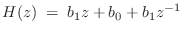 which is real for all
 .
.
- Extending the previous example, every order
 zero-phase real FIR
filter has an impulse response of the form
zero-phase real FIR
filter has an impulse response of the form
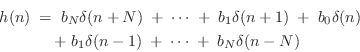
and frequency response
which is clearly real whenever the coefficients
 are real.
- There is no first-order (length 2) zero-phase filter, because,
to be even, its impulse response would have to be proportional to
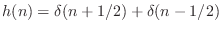 . Since the bandlimited digital
impulse signal
. Since the bandlimited digital
impulse signal  is ideally interpolated using bandlimited
interpolation [91,84], giving samples of
sinc
is ideally interpolated using bandlimited
interpolation [91,84], giving samples of
sinc --the
unit-amplitude sinc function having zero-crossings on the
integers, we see that sampling
--the
unit-amplitude sinc function having zero-crossings on the
integers, we see that sampling  on the integers yields
an IIR filter:
on the integers yields
an IIR filter:
 sinc
sinc sinc
sinc
- Similarly, there are no odd-order (even-length) zero-phase filters.
Odd Impulse Reponses
Note that odd impulse responses of the form
![]() are
closely related to zero-phase filters (even impulse responses). This
is because another Fourier symmetry relation is that the DTFT of an
odd sequence is purely imaginary [84]. In
practice, Hilbert transform filters and differentiators
are often implemented as odd FIR filters [68]. A
purely imaginary frequency response can be divided by
are
closely related to zero-phase filters (even impulse responses). This
is because another Fourier symmetry relation is that the DTFT of an
odd sequence is purely imaginary [84]. In
practice, Hilbert transform filters and differentiators
are often implemented as odd FIR filters [68]. A
purely imaginary frequency response can be divided by ![]() to give a
real frequency response. As a result, filter-design software for one
case is easily adapted to the other [68].
to give a
real frequency response. As a result, filter-design software for one
case is easily adapted to the other [68].
Equivalently, an odd impulse response can be multiplied by ![]() in the
time domain to yield a purely imaginary impulse response that
is Hermitian. Hermitian signals have real Fourier
transforms [84]. Therefore, a Hermitian impulse response gives
a filter having a phase response that is either zero or
in the
time domain to yield a purely imaginary impulse response that
is Hermitian. Hermitian signals have real Fourier
transforms [84]. Therefore, a Hermitian impulse response gives
a filter having a phase response that is either zero or ![]() at each
frequency.
at each
frequency.
Symmetric Linear-Phase Filters
As stated at the beginning of this chapter, the impulse response of every causal, linear-phase, FIR filter is symmetric:

Simple Linear-Phase Filter Examples
- The example of §10.2.1 was in fact a linear-phase FIR
filter design example. The resulting causal finite impulse response
was left-shifted (``advanced'' in time) to make it zero phase.
- While the trivial ``bypass filter''
is zero-phase
(§10.2.2), the ``bypass filter with a unit delay,''
 is linear phase. It is (trivially) symmetric
about time
is linear phase. It is (trivially) symmetric
about time  , and the frequency response is
 , which
is a pure linear phase term
, which
is a pure linear phase term
 having a slope
of
having a slope
of  samples (radians per radians-per-sample), or
  seconds
(radians per radians-per-second). The phase- and group-delays are
each 1 sample at every frequency.
seconds
(radians per radians-per-second). The phase- and group-delays are
each 1 sample at every frequency.
- The impulse response of the simplest lowpass filter studied in
Chapter 1 was
 [
[
 ].
Since this impulse response is symmetric about time
].
Since this impulse response is symmetric about time  samples,
it is linear phase, and
samples,
it is linear phase, and
 , as derived
in Chapter 1. The phase delay and group delay are both
, as derived
in Chapter 1. The phase delay and group delay are both  sample at
each frequency. Note that even-length linear-phase filters cannot be
time-shifted (without interpolation) to create a corresponding
zero-phase filter. However, they can be shifted to make a
near-zero-phase filter that has a phase delay and group delay equal to
half a sample at all passband frequencies.
sample at
each frequency. Note that even-length linear-phase filters cannot be
time-shifted (without interpolation) to create a corresponding
zero-phase filter. However, they can be shifted to make a
near-zero-phase filter that has a phase delay and group delay equal to
half a sample at all passband frequencies.
Software for Linear-Phase Filter Design
The Matlab Signal Processing Toolbox covers many applications with the following functions:
![$\displaystyle \begin{tabular}{rl}
\texttt{remez()} & (optimal Chebyshev linear-...
...or general FIR (or IIR)\\
& filter design \cite[page 50]{JOST}).
\end{tabular}$](http://www.dsprelated.com/josimages_new/filters/img1217.png)
Methods for FIR filter design are discussed in the fourth book of the music signal processing series [87], and classic references include [64,68]. There is also quite a large research literature on this subject.
Antisymmetric Linear-Phase Filters
In the same way that odd impulse responses are related to even impulse
responses, linear-phase filters are closely related
to antisymmetric impulse responses of the form
![]() ,
, ![]() . An antisymmetric impulse response is
simply a delayed odd impulse response (usually delayed enough to make
it causal). The corresponding frequency response is not strictly
linear phase, but the phase is instead linear with a constant offset
(by
. An antisymmetric impulse response is
simply a delayed odd impulse response (usually delayed enough to make
it causal). The corresponding frequency response is not strictly
linear phase, but the phase is instead linear with a constant offset
(by ![]() ). Since an affine function is any function of
the form
). Since an affine function is any function of
the form
![]() , where
, where ![]() and
and ![]() are constants, an antisymmetric impulse response can be called an
affine-phase filter. These same remarks apply to any linear-phase
filter that can be expressed as a time-shift of a
are constants, an antisymmetric impulse response can be called an
affine-phase filter. These same remarks apply to any linear-phase
filter that can be expressed as a time-shift of a ![]() -phase filter
(i.e., it is inverting in some passband). However, in practice, all
such filters may be loosely called ``linear-phase'' filters, because
they are designed and implemented in essentially the same
way [68].
-phase filter
(i.e., it is inverting in some passband). However, in practice, all
such filters may be loosely called ``linear-phase'' filters, because
they are designed and implemented in essentially the same
way [68].
Note that truly linear-phase filters have both a constant phase delay and a constant group delay. Affine-phase filters, on the other hand, have a constant group delay, but not a constant phase delay.
Forward-Backward Filtering
There are no linear-phase recursive filters because a recursive filter
cannot generate a symmetric impulse response. However,
it is possible to implement a zero-phase filter offline
using a recursive filter twice. That is, if the entire input signal
![]() is stored in a computer memory or hard disk, for example,
then we can apply a recursive filter both forward and backward in
time. Doing this squares the amplitude response of the filter
and zeros the phase response.
is stored in a computer memory or hard disk, for example,
then we can apply a recursive filter both forward and backward in
time. Doing this squares the amplitude response of the filter
and zeros the phase response.
To show this analytically, let ![]() denote the output of the first
filtering operation (which we'll take to be ``forward'' in time in the
normal way), and let
denote the output of the first
filtering operation (which we'll take to be ``forward'' in time in the
normal way), and let ![]() be the impulse response of the recursive
filter. Then we have
be the impulse response of the recursive
filter. Then we have
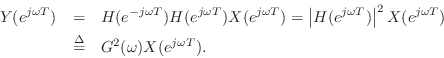
Using this result and applying the convolution theorem (§6.3) twice gives the z transform
If the filter were complex, then we would need to conjugate its coefficients when running it backwards.
In summary, we have thus shown that forward-backward
filtering squares the amplitude response and zeros the
phase response. Note also that the phase response is truly zero,
never alternating between zero and ![]() . No matter what nonlinear
phase response
. No matter what nonlinear
phase response
![]() a filter may have, this phase is
completely canceled out by forward and backward filtering. The
amplitude response, on the other hand, is squared. For simple
bandpass filters (including lowpass, highpass, etc.), for which the
desired gain is 1 in the passband and 0 in the stopband, squaring the
amplitude response usually improves the response, because the
``stopband ripple'' (deviation from 0) is squared,
thereby doubling the stopband attenuation in dB. On the other
hand, passband ripple (deviation from 1) is only doubled by the
squaring (because
a filter may have, this phase is
completely canceled out by forward and backward filtering. The
amplitude response, on the other hand, is squared. For simple
bandpass filters (including lowpass, highpass, etc.), for which the
desired gain is 1 in the passband and 0 in the stopband, squaring the
amplitude response usually improves the response, because the
``stopband ripple'' (deviation from 0) is squared,
thereby doubling the stopband attenuation in dB. On the other
hand, passband ripple (deviation from 1) is only doubled by the
squaring (because
![]() ).
).
A Matlab example of forward-backward filtering is presented in §11.6 (in Fig.11.1).
Phase Distortion at Passband Edges
For many applications (such as lowpass, bandpass, or highpass
filtering), the most phase dispersion occurs at the extreme
edge of the passband (i.e., in the vicinity of cut-off
frequencies). This phenomenon was clearly visible in the example
of Fig.7.6.4. Only filters without feedback can have
exactly linear phase (unless forward-backward filtering is feasible),
and such filters generally need many more multiplies for a given
specification on the amplitude response
![]() [68]. One should keep in mind that phase
dispersion near a cut-off frequency (or any steep transition in the
amplitude response) usually appears as ringing near that
frequency in the time domain. (This can be heard in the upcoming
matlab example of §11.6, Fig.11.1.)
[68]. One should keep in mind that phase
dispersion near a cut-off frequency (or any steep transition in the
amplitude response) usually appears as ringing near that
frequency in the time domain. (This can be heard in the upcoming
matlab example of §11.6, Fig.11.1.)
For musical purposes, ![]() , or the effect that a filter has on
the magnitude spectrum of the input signal, is usually of primary
interest. This is true for all ``instantaneous'' filtering operations
such as tone controls, graphical equalizers, parametric equalizers,
formant filter banks, shelving filters, and the like. (Elementary
examples in this category are discussed in Appendix B.)
Notable exceptions are echo and reverberation [86], in which
delay characteristics are as important as magnitude characteristics.
, or the effect that a filter has on
the magnitude spectrum of the input signal, is usually of primary
interest. This is true for all ``instantaneous'' filtering operations
such as tone controls, graphical equalizers, parametric equalizers,
formant filter banks, shelving filters, and the like. (Elementary
examples in this category are discussed in Appendix B.)
Notable exceptions are echo and reverberation [86], in which
delay characteristics are as important as magnitude characteristics.
When designing an ``instantaneous'' filtering operation, i.e., when not
designing a ``delay effect'' such as an echo unit or reverberator, the
amplitude response ![]() should be as smooth as possible
as a function of frequency
should be as smooth as possible
as a function of frequency ![]() . Smoother amplitude responses
correspond to shorter impulse responses (when the phase is zero,
linear, or ``minimum phase'' as discussed in the next chapter). By
keeping impulse-responses as short as possible, phase dispersion is
minimized, and ideally inaudible. Linearizing the phase response with
a delay equalizer (a type of allpass filter) does not eliminate
ringing, but merely shifts it in time. A general rule of thumb is to
keep the total impulse-response duration below the time-discrimination
threshold of hearing in the context of the intended application.
. Smoother amplitude responses
correspond to shorter impulse responses (when the phase is zero,
linear, or ``minimum phase'' as discussed in the next chapter). By
keeping impulse-responses as short as possible, phase dispersion is
minimized, and ideally inaudible. Linearizing the phase response with
a delay equalizer (a type of allpass filter) does not eliminate
ringing, but merely shifts it in time. A general rule of thumb is to
keep the total impulse-response duration below the time-discrimination
threshold of hearing in the context of the intended application.
Next Section:
Minimum-Phase Filters
Previous Section:
Implementation Structures for Recursive Digital Filters


