


Peak Detection (Steps 3 and 4)
Due to the sampled nature of spectra obtained using the STFT, each
peak (location and height) found by finding the maximum-magnitude
frequency bin is only accurate to within half a bin. A bin represents
a frequency interval of ![]() Hz, where
Hz, where ![]() is the FFT size.
Zero-padding increases the number of FFT bins per Hz and thus
increases the accuracy of the simple peak detection. However, to
obtain frequency accuracy on the level of
is the FFT size.
Zero-padding increases the number of FFT bins per Hz and thus
increases the accuracy of the simple peak detection. However, to
obtain frequency accuracy on the level of ![]() of the distance
from a sinc maximum to its first zero crossing (in the case of a
rectangular window), the zero-padding factor required is
of the distance
from a sinc maximum to its first zero crossing (in the case of a
rectangular window), the zero-padding factor required is ![]() .
(Note that with no zero padding, the STFT analysis parameters are
typically arranged so that the distance from the sinc peak to its
first zero-crossing is equal to the fundamental frequency of a
harmonic sound. Under these conditions,
.
(Note that with no zero padding, the STFT analysis parameters are
typically arranged so that the distance from the sinc peak to its
first zero-crossing is equal to the fundamental frequency of a
harmonic sound. Under these conditions, ![]() of this interval is
equal to the relative accuracy in the fundamental frequency
measurement. Thus, this is a realistic specification in view of pitch
discrimination accuracy.) Since we would nominally take two periods
into the data frame (for a Rectangular window), a
of this interval is
equal to the relative accuracy in the fundamental frequency
measurement. Thus, this is a realistic specification in view of pitch
discrimination accuracy.) Since we would nominally take two periods
into the data frame (for a Rectangular window), a ![]() Hz sinusoid
at a sampling rate of
Hz sinusoid
at a sampling rate of ![]() KHz would have a period of
KHz would have a period of
![]() samples, so that the FFT size would have to exceed
one million. A more efficient spectral interpolation scheme is to
zero-pad only enough so that quadratic (or other simple) spectral
interpolation, using only bins immediately surrounding the
maximum-magnitude bin, suffices to refine the estimate to
samples, so that the FFT size would have to exceed
one million. A more efficient spectral interpolation scheme is to
zero-pad only enough so that quadratic (or other simple) spectral
interpolation, using only bins immediately surrounding the
maximum-magnitude bin, suffices to refine the estimate to ![]() accuracy. PARSHL uses a parabolic interpolator which fits a parabola
through the highest three samples of a peak to estimate the true peak
location and height (cf. Fig.H.2).
accuracy. PARSHL uses a parabolic interpolator which fits a parabola
through the highest three samples of a peak to estimate the true peak
location and height (cf. Fig.H.2).
![\includegraphics[width=\twidth]{eps/fig4}](http://www.dsprelated.com/josimages_new/sasp2/img3048.png)
![\includegraphics[width=\twidth]{eps/fig5}](http://www.dsprelated.com/josimages_new/sasp2/img3049.png)
We have seen that each sinusoid appears as a shifted window transform which is a sinc-like function. A robust method for estimating peak frequency with very high accuracy would be to fit a window transform to the sampled spectral peaks by cross-correlating the whole window transform with the entire spectrum and taking and interpolated peak location in the cross-correlation function as the frequency estimate. This method offers much greater immunity to noise and interference from other signal components.
To describe the parabolic interpolation strategy, let's define a
coordinate system centered at
![]() , where
, where ![]() is the bin
number of the spectral magnitude maximum, i.e.,
is the bin
number of the spectral magnitude maximum, i.e.,
![]() for all
for all
![]() . An example is shown in
Figure 4. We desire a general parabola of the form
. An example is shown in
Figure 4. We desire a general parabola of the form
 |
(H.2) |
such that
 |
(H.3) | ||
 |
(H.4) | ||
 |
(H.5) |
We have found empirically that the frequencies tend to be about twice as accurate when dB magnitude is used rather than just linear magnitude. An interesting open question is what is the optimum nonlinear compression of the magnitude spectrum when quadratically interpolating it to estimate peak locations.
Solving for the parabola peak location ![]() , we get
, we get
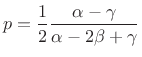 |
(H.6) |
and the estimate of the true peak location (in bins) will be
 |
(H.7) |
and the peak frequency in Hz is
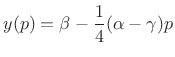 |
(H.8) |
The magnitude spectrum is used to find
Once an interpolated peak location has been found, the entire local maximum in the spectrum is removed. This allows the same algorithm to be used for the next peak. This peak detection and deletion process is continued until the maximum number of peaks specified by the user is found.
Next Section:
Peak Matching (Step 5)
Previous Section:
Filling the FFT Input Buffer (Step 2)


